Dealing with Dynamic States
Measurement outcomes are rarely static over time. They will possess a dynamic component that must be understood for correct interpretation of the results. For example, a trace made on an ink pen chart recorder will be subject to the speed at which the pen can follow the input signal changes.
To properly appreciate instrumentation design and its use, it is now necessary to develop insight into the most commonly encountered types of dynamic response and to develop the mathematical modelling basis that allows us to make concise statements about responses.
If the transfer relationship for a block follows linear laws of performance, then a generic mathematical method of dynamic description can be used. Unfortunately, simple mathematical methods have not been found that can describe all types of instrument responses in a simplistic and uniform manner. If the behavior is nonlinear, then description with mathematical models becomes very difficult and might be impracticable. The behavior of nonlinear systems can, however, be studied as segments of linear behavior joined end to end. Here, digital computers are effectively used to model systems of any kind provided the user is prepared to spend time setting up an adequate model.
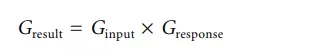
Now the mathematics used to describe linear dynamic systems can be introduced. This gives valuable insight into the expected behavior of instrumentation, and it is usually found that the response can be approximated as linear. The modelled response at the output of a block Gresult is obtained by multiplying the mathematical expression for the input signal Ginput by the transfer function of the block under investigation Gresponse , as shown in Equation 3.5.
To proceed, one needs to understand commonly encountered input functions and the various types of block characteristics. We begin with the former set: the so-called forcing functions.
Forcing Functions
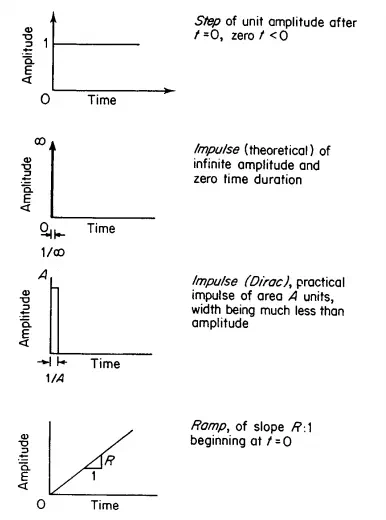
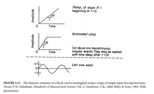
Let us first develop an understanding of the various types of input signal used to perform tests. The most commonly used signals are shown in Figure 3.12. These each possess different valuable test features. For example, the sine-wave is the basis of analysis of all complex wave-shapes because they can be formed as a combination of various sine-waves, each having individual responses that add to give all other waveshapes. The step function has intuitively obvious uses because input transients of this kind are commonly encountered. The ramp test function is used to present a more realistic input for those systems where it is not possible to obtain instantaneous step input changes, such as attempting to move a large mass by a limited size of force. Forcing functions are also chosen because they can be easily described by a simple mathematical expression, thus making mathematical analysis relatively straightforward.
Characteristic Equation Development
The behavior of a block that exhibits linear behavior is mathematically represented in the general form of expression given as Equation 3.6.

Here, the coefficients a2, a1, and a0 are constants dependent on the particular block of interest. The left-hand side of the equation is known as the characteristic equation. It is specific to the internal properties of the block and is not altered by the way the block is used.
The specific combination of forcing function input and block characteristic equation collectively decides the combined output response. Connections around the block, such as feedback from the output to the input, can alter the overall behavior significantly: such systems, however, are not dealt with in this section being in the domain of feedback control systems.
Solution of the combined behavior is obtained using Laplace transform methods to obtain the output responses in the time or the complex frequency domain. These mathematical methods might not be familiar to the reader, but this is not a serious difficulty for the cases most encountered in practice are
well documented in terms that are easily comprehended, the mathematical process having been performed to yield results that can be used without the same level of mathematical ability. More depth of explanation can be obtained from [1] or any one of the many texts on energy systems analysis. Space here only allows an introduction; this account is linked to [1], Chapter 17, to allow the reader to access a fuller description where needed.
The next step in understanding block behavior is to investigate the nature of Equation 3.6 as the number of derivative terms in the expression increases, Equations 3.7 to 3.10.
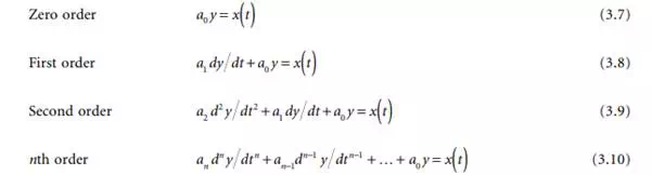
Note that specific names have been given to each order. The zero-order situation is not usually dealt with in texts because it has no time-dependent term and is thus seen to be trivial. It is an amplifier (or attenuator) of the forcing function with gain of a0. It has infinite bandwidth without change in the amplification constant.
The highest order usually necessary to consider in first-cut instrument analysis is the second-order class. Higher-order systems do occur in practice and need analysis that is not easily summarized here. They also need deep expertise in their study. Computer-aided tools for systems analysis can be used to study the responses of systems.
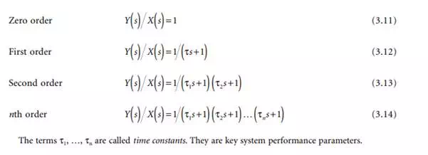
Another step is now to rewrite the equations after Laplace transformation into the frequency domain. We then get the set of output/input Equations 3.11 to 3.14.
Response of the Different Linear Systems Types
Space restrictions do not allow a detailed study of all of the various options. A selection is presented to show how they are analysed and reported, that leading to how the instrumentation person can use certain standard charts in the study of the characteristics of blocks.
Zero-Order Blocks
To investigate the response of a block, multiply its frequency domain forms of equation for the characteristic equation with that of the chosen forcing function equation.
This is an interesting case because Equation 3.7 shows that the zero-order block has no frequency dependent term (it has no time derivative term), so the output for all given inputs can only be of the same time form as the input. What can be changed is the amplitude given as the coefficient a0. A shift in time (phase shift) of the output waveform with the input also does not occur as it can for the higher-order blocks.
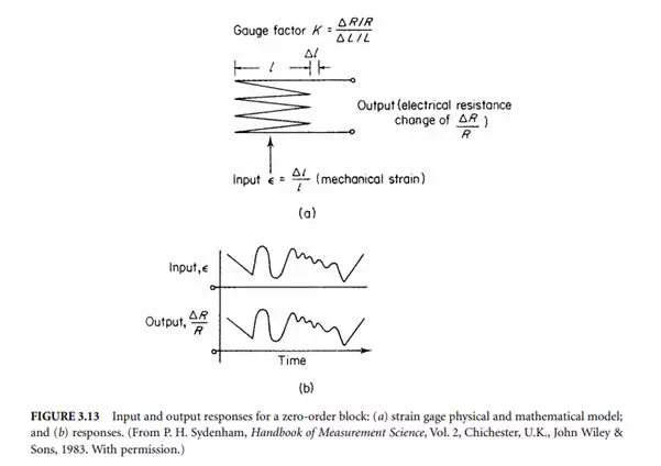
This is the response often desired in instruments because it means that the block does not alter the time response. However, this is not always so because, in systems, design blocks are often chosen for their ability to change the time shape of signals in a known manner.
Although somewhat obvious, Figure 3.13, a resistive strain gage, is given to illustrate zero-order behavior.
First-Order Blocks
Here, Equation 3.8 is the relevant characteristic equation. There is a time-dependent term, so analysis is needed to see how this type of block behaves under dynamic conditions. The output response is different for each type of forcing function applied. Space limitations only allow the most commonly encountered cases — the step and the sine-wave input — to be introduced here. It is also only possible here to outline the method of analysis and to give the standardized charts that plot generalized behavior.
The step response of the first-order system is obtained by multiplying Equation 3.12 by the frequency domain equation for a step of amplitude A. The result is then transformed back into the time domain using Laplace transforms to yield the expression for the output, y(t)

where A is the amplitude of the step, K the static gain of the first-order block, t the time in consistent units, and τ the time constant associated with the block itself.
This is a tidy outcome because Equation 3.15 covers the step response for all first-order blocks, thus allowing it to be graphed in normalized manner, as given in Figure 3.14. The shape of the response is always of the same form. This means that the step response of a first-order system can be described as having “a step of AK amplitude with the time constant τ.

If the input is a sine-wave, the output response is quite different; but again, it will be found that there is a general solution for all situations of this kind. As before, the input forcing equation is multiplied by the characteristic equation for the first-order block and Laplace transformation is used to get back to the time domain response. After rearrangement into two parts, this yields:

where ω is the signal frequency in angular radians, φ = tan–1 (–ωt), A the amplitude of the sine-wave input, K the gain of the first-order block, t the time in consistent units, and τ the time constant associated with the block.
The left side of the right-hand bracketed part is a short-lived, normally ignored, time transient that rapidly decays to zero, leaving a steady-state output that is the parameter of usual interest. Study of the steady-state part is best done by plotting it in a normalized way, as has been done in Figure 3.15. These plots show that the amplitude of the output is always reduced as the frequency of the input signal rises and that there is always a phase lag action between the input and the output that can range from 0 to 90° but never be more than 90°. The extent of these effects depends on the particular coefficients of the block and input signal. These effects must be well understood when interpreting measurement results because substantial errors can arise with using first-order systems in an instrument chain.


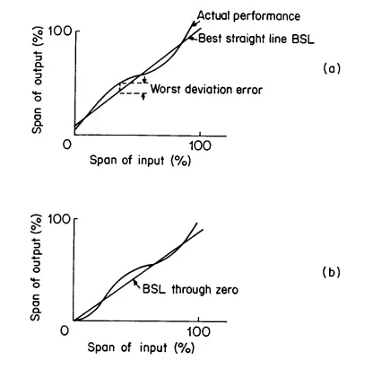
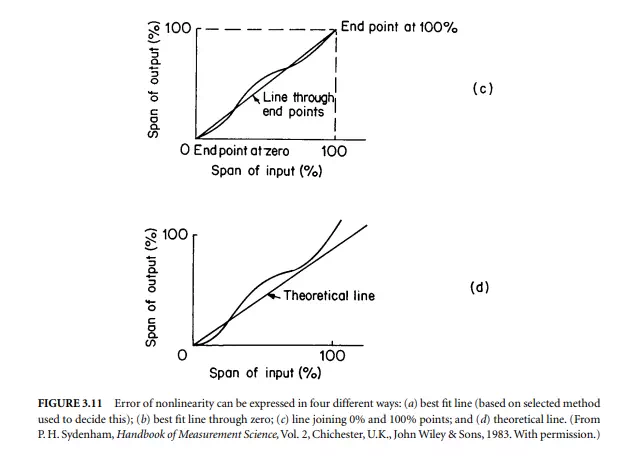
Comments are closed.