The null method is one possible mode of operation for a measuring instrument. A null instrument uses the null method for measurement. In this method, the instrument exerts an influence on the measured system so as to oppose the effect of the measurand. The influence and the measurand are balanced until they are equal but opposite in value, yielding a null measurement. Typically, this is accomplished by some type of feedback operation that allows the comparison of the measurand against a known standard value. Key features of a null instrument include: an iterative balancing operation using some type of comparator, either a manual or automatic feedback used to achieve balance, and a null deflection at parity.

A null instrument offers certain intrinsic advantages over other modes of operation (e.g., see deflection instruments). By balancing the unknown input against a known standard input, the null method minimizes interaction between the measuring system and the measurand. As each input comes from a separate source, the significance of any measuring influence on the measurand by the measurement process is reduced. In effect, the measured system sees a very high input impedance, thereby minimizing loading errors. This is particularly effective when the measurand is a very small value. Hence, the null operation can achieve a high accuracy for small input values and a low loading error. In practice, the null instrument will not achieve perfect parity due to the usable resolution of the balance and detection methods, but this is limited only by the state of the art of the circuit or scheme being employed.

A disadvantage of null instruments is that an iterative balancing operation requires more time to execute than simply measuring sensor input. Thus, this method might not offer the fastest measurement possible when high-speed measurements are required. However, the user should weigh achievable accuracy against needed speed of measurement when considering operational modes. Further, the design of the comparator and balance loop can become involved such that highly accurate devices are generally not the lowest cost measuring alternative.

An equal arm balance scale is a good mechanical example of a manual balance-feedback null instrument, as shown in Figure 2.1. This scale compares the unknown weight of an object on one side against a set of standard or known weights. Known values of weight are iteratively added to one side to exert an influence to oppose the effect of the unknown weight on the opposite side. Until parity, a high or low value is noted by the indicator providing the feedback logic to the operator for adding or removing

weights in a balancing iteration. At true parity, the scale indicator is null; that is, it indicates a zero deflection. Then, the unknown input or measurand is deduced to have a value equal to the balance input, the amount of known weights used to balance the scale. Factors influencing the overall measurement accuracy include the accuracy of the standard weights used and resolution of the output indicator, and the friction at the fulcrum. Null instruments exist for measurement of most variables. Other common examples include bridge circuits, often employed for highly accurate resistance measurements and found in load cells, temperature-compensated transducers, and voltage balancing potentiometers used for highly accurate low-voltage measurements.

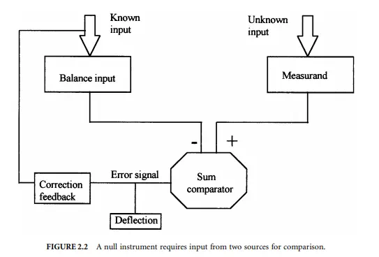
Within the null instrument, the iteration and feedback mechanism is a loop that can be controlled either manually or automatically. Essential to the null instrument are two inputs: the measurand and the balance input. The null instrument includes a differential comparator, which compares and computes the difference between these two inputs. This is illustrated in Figure 2.2. A nonzero output from the comparator provides the error signal and drives the logic for the feedback correction. Repeated corrections provide for an iteration toward eventual parity between the inputs and results in the null condition where the measurand is exactly opposed by the balance input. At parity, the error signal is driven to zero by the opposed influence of the balance input and the indicated deflection is at null, thus lending the name to the method. It is the magnitude of the balance input that drives the output reading in terms of the measurand.

Deflection Instrument

The deflection method is one possible mode of operation for a measuring instrument. A deflection instrument uses the deflection method for measurement. A deflection instrument is influenced by the measurand so as to bring about a proportional response within the instrument. This response is an output reading that is a deflection or a deviation from the initial condition of the instrument. In a typical form, the measurand acts directly on a prime element or primary circuit so as to convert its information into a detectable form. The name is derived from a common form of instrument where there is a physical deflection of a prime element that is linked to an output scale, such as a pointer or other type of readout, which deflects to indicate the measured value. The magnitude of the deflection of the prime element brings about a deflection in the output scale that is designed to be proportional in magnitude to the value of the measurand.

Deflection instruments are the most common of measuring instruments. The relationship between the measurand and the prime element or measuring circuit can be a direct one, with no balancing mechanism or comparator circuits used. The proportional response can be manipulated through signal conditioning methods between the prime element and the output scale so that the output reading is a direct indication of the measurand. Effective designs can achieve a high accuracy, yet sufficient accuracy for less demanding uses can be achieved at moderate costs.

An attractive feature of the deflection instrument is that it can be designed for either static or dynamic measurements or both. An advantage to deflection design for dynamic measurements is in the high dynamic response that can be achieved. A disadvantage of deflection instruments is that by deriving its energy from the measurand, the act of measurement will influence the measurand and change the value of the variable being measured. This change is called a loading error. Hence, the user must ensure that the resulting error is acceptable. This usually involves a careful look at the instrument input impedance for the intended measurement.

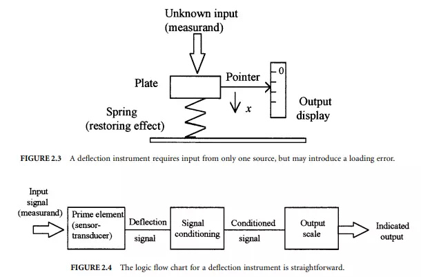
A spring scale is a good, simple example of a deflection instrument. As shown in Figure 2.3, the input weight or measurand acts on a plate-spring. The plate-spring serves as a prime element. The original position of the spring is influenced by the applied weight and responds with a translational displacement, a deflection x. The final value of this deflection is a position that is at equilibrium between the downward force of the weight, and the upward restoring force of the spring, kx. That is, the input force is balanced against the restoring force. A mechanical coupler is connected directly or by linkage to a pointer. The pointer position is mapped out on a corresponding scale that serves as the readout scale. For example, at equilibrium W = kx or by measuring the deflection of the pointer the weight is deduced by x = W/k.

The flow diagram logic for a deflection instrument is rather linear, as shown if Figure 2.4. The input signal is sensed by the prime element or primary circuit and thereby deflected from its initial setting. The deflection signal is transmitted to signal conditioners that act to condition the signal into a desired form. Examples of signal conditioning are to multiply the deflection signal by some scaler magnitude, such as in amplification or filtering, or to transform the signal by some arithmetic function. The conditioned signal is then transferred to the output scale, which provides the indicated value corresponding to the measurand value.

Analog and Digital Sensors

Analog sensors provide a signal that is continuous in both its magnitude and its temporal (time) or spatial (space) content. The defining word for analog is “continuous.” If a sensor provides a continuous output signal that is directly proportional to the input signal, then it is analog.

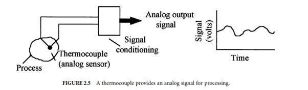
Most physical variables, such as current, temperature, displacement, acceleration, speed, pressure, light intensity, and strain, tend to be continuous in nature and are readily measured by an analog sensor and represented by an analog signal. For example, the temperature within a room can take on any value within its range, will vary in a continuous manner in between any two points in the room, and may vary continuously with time at any position within the room. An analog sensor, such as a bulb thermometer or a thermocouple, will continuously respond to such temperature changes. Such a continuous signal is shown in Figure 2.5, where the signal magnitude is analogous to the measured variable (temperature) and the signal is continuous in both magnitude and time. Digital sensors provide a signal that is a direct digital representation of the measurand.

Digital sensors are basically binary (“on” or “off”) devices. Essentially, a digital signal exists at only discrete values of

time (or space). And within that discrete period, the signal can represent only a discrete number of magnitude values. A common variation is the discrete sampled signal representation, which represents a sensor output in a form that is discrete both in time or space and in magnitude.

Digital sensors use some variation of a binary numbering system to represent and transmit the signal information in digital form.A binary numbering system is a number system using the base 2. The simplest binary signal is a single bit that has only one of two possible values, a 1 or a 0. Bits are like electrical “on-off” switches and are used to convey logical and numerical information. With appropriate input, the value of the bit transmitted is reset corresponding to the behavior of the measured variable. A digital sensor that transmits information one bit at a time uses serial transmission. By combining bits or transmitting bits in groups, it is also possible to define logical commands or integer numbers beyond a 0 or 1. A digital sensor that transmits bits in groups uses parallel transmission. With any digital device, an M-bit signal can express 2M different numbers. This also provides the limit for the different values that a digital device can discern. For example, a 2-bit device can express 22 or 4 different numbers, 00, 01, 10, and 11, corresponding to the values of 0, 1, 2, and 3, respectively. Thus, the resolution in a magnitude discerned by a digital sensor is inherently limited to 1 part in 2M.

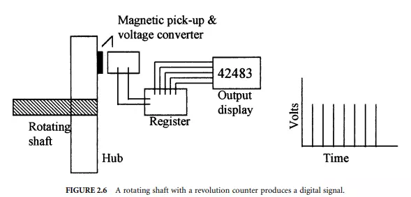
The concept of a digital sensor is illustrated by the revolution counter in Figure 2.6. Such devices are widely used to sense the revolutions per minute of a rotating shaft. In this example, the sensor is a magnetic pick-up/voltage converter that outputs a pulse with each pass of a magnetic stud mounted to a hub on the rotating shaft. The output from the pick-up normally is “off” but is momentarily turned “on” by the passing stud. This pulse is a voltage spike sent to a digital register whose value is increased by a single count with each spike. The register can send the information to an output device, such as the digital display shown. The output from the sensor can be viewed in terms of voltage spikes with time. The count rate is related to the rotational speed of the shaft. As seen, the signal is discrete in time. A single stud with pick-up will increase the count by one for each full rotation of the shaft. Fractions of a rotation can be resolved by increasing the number of studs on the hub. In this example, the continuous rotation of the shaft is analog, but the revolution count is digital. The amplitude of the voltage spike is set to activate the counter and is not related to the shaft rotational speed.