A plot of the concentration profile (normalized with respect to Cs) , at various times, is given here.
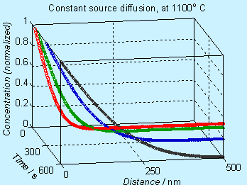

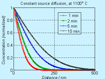
Figure 6.2. Concentration profile for doping by constant source diffusion
Note that the concentration axis is in linear scale. Many times, the concentration axis is in log scale and the figures will appear to be different, as shown below.
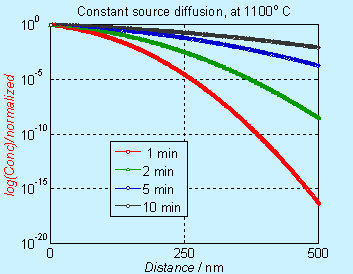
Figure 6.3. Concentration profile for doping by constant source diffusion (log scale)
Limited source diffusion: In the second mode of diffusion called limited source or drive in diffusion, we assume that the source is a limited quantity of dopant, all concentrated at the surface. Thus, the quantity QT is given by ![]()
This is a reasonable approximation as long as the dopant is mostly restricted to the surface, in the beginning.
At any t >0, the total dopant inside the wafer is given by QT and this is given by ![]()
Similalry, the source is removed at t=0, and there is no flux ![]() of dopant from outside, for t > 0. Initially (t=0), the concentration of dopant inside the surface (except on the surface) is zero. The concentration at a location too far away from the surface (inside the wafer) is zero.
of dopant from outside, for t > 0. Initially (t=0), the concentration of dopant inside the surface (except on the surface) is zero. The concentration at a location too far away from the surface (inside the wafer) is zero.
These are reflected in the following equations. 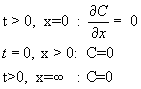
It can be shown that the following Gaussian profile satisfies the differential equation and the boundary conditions. ![]()
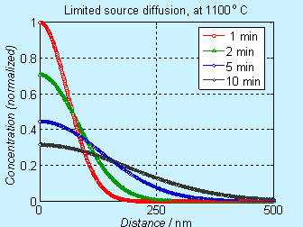
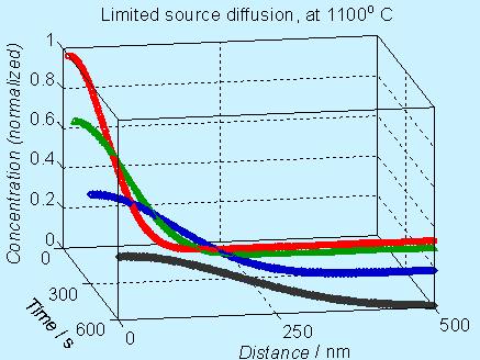
Figure 6.4. Concentration profile for doping by limited source diffusion
In log scale, the concentration profile appear to be different, as shown below.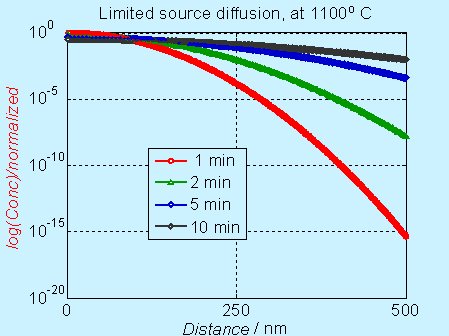
Figure 6.5. Concentration profile for doping by limited source diffusion (log scale)
Near the surface, the concentration decreases significantly with time, but it is not obvious in the log scale. The complementary error function (constant source diffusion) is a decreases faster compared to the Gaussian function (limited source diffusion). This is illustrated in the figure below.
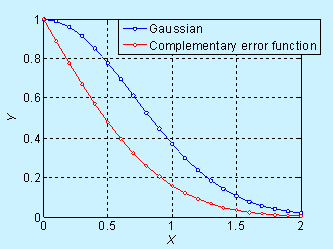
Figure 6.6. Comparison of concentration profile for doping by constant source diffusion and limited source diffusion
In log scale, it is given below
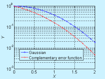
Figure 6.6. Comparison of concentration profile for doping by constant source diffusion and limited source diffusion (log scale)
Solubility: The solubility of a dopant in the substrate also plays a key role. Even if the diffusivity is large, if the solubility is small, then it will take a long time to achieve a particular level of doping. This is because the total quantity diffused depends on the concentration gradient and the diffusivity. The concentration gradient depends on the solubility limit. Typically, the solubility of dopant is much more than the doping level required. The solubility is a function of temperature and for most dopants, it varies between 1019 to 1021 atoms-cm-3 in the temperature range of 400 -1000 ˚C. For impurities such as Cu, Fe or Au, the solubility is in the range of 1015 to 1018 atoms-cm-3 in the same temperature range. At 1000 ˚C, the diffusivity of As in Si is in the range of 10-15 cm2/s, B in Si is in the range of 10-14 cm2/s and P in Si is in the range of 5 ×10-15 cm2/s. On the other hand, the diffusivities of some of the contaminants are much higher. For example, in Si at 500 – 1000 ˚C range, the diffusivity of Cu, Fe and Au are in the range of 10-2 to 10-7 cm2/s.
Equipment: Usually, large chambers that can hold many wafers are used to conduct the diffusion process. The doping source is usually in gas or liquid phase. When it is a liquid source, it is typically carried out using nitrogen in gaseous form; that is, the carrier gas will be bubbled through the liquid source. Sometimes even for solid source the carrier gas may pass over a heated solid source. The inert gas is used so that it can provide enough volume and maintain a laminar flow. Even though liquid or gas sources are used, finally they are all converted to solid source. For example, if phosphorus oxy-chloride is used as a source, it will react with oxygen and form phosphorus pentoxide, which will be deposited on top of the wafer. If phosphine is used, that will also be reacted with oxygen, so that phosphorus pentoxide can form on the wafer.
When a solid source is used, the source will be in the form of slugs, which will be kept between the wafers. There are some advantages and disadvantages. The advantage is that these are safer to handle. There is no toxic wafer, at least at room temperature. The disadvantage is that cleaning is an issue; the slugs can break down, in which case, cleaning is an issue. The other disadvantage is the throughput is low; that is, the number of wafers that can be doped in unit time is lower in this method.
Comments are closed.