There is a little distinction between variable-reluctance and variable-inductance transducers. Mathematically, the principles of linear-variable inductors are very similar to the variable-reluctance type of transducer. The distinction is mainly in the pickups rather than principles of operations. A typical linear variable inductor consists of a movable iron core that provides the mechanical input and two coils forming two legs of a bridge network. A typical example of such a transducer is the variable coupling transducer, which is discussed next.
Variable-Coupling Transducers
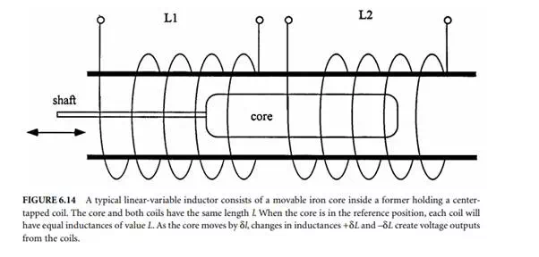
These transducers consist of a former holding a centre tapped coil and a ferromagnetic plunger, as shown in Figure 6.14.
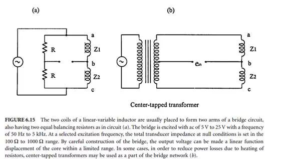
The plunger and the two coils have the same length l. As the plunger moves, the inductances of the coils change. The two inductances are usually placed to form two arms of a bridge circuit with two equal balancing resistors, as shown in Figure 6.15. The bridge is excited with ac of 5 V to 25 V with a frequency of 50 Hz to 5 kHz. At the selected excitation frequency, the total transducer impedance at null conditions is set in the 100 Ω to 1000 Ω range. The resistors are set to have about the same value as transducer impedances. The load for the bridge output must be at least 10 times the resistance, R, value. When the plunger is in the reference position, each coil will have equal inductances of value L.As the plunger moves by δL, changes in inductances +δL and –δL creates a voltage output from the bridge. By constructing the bridge carefully, the output voltage can be made as a linear function displacement of the moving plunger within a rated range.
In some transducers, in order to reduce power losses due to heating of resistors, centre-tapped transformers can be used as a part of the bridge network, as shown in Figure 6.15(b). In this case, the circuit becomes more inductive and extra care must be taken to avoid the mutual coupling between the transformer and the transducer.
It is particularly easy to construct transducers of this type, by simply winding a center-tapped coil on a suitable former. The variable-inductance transducers are commercially available in strokes from about 2 mm to 500 cm. The sensitivity ranges between 1% full scale to 0.02% in long stroke special constructions. These devices are also known as linear displacement transducers or LDTs, and they are available in various shape and sizes.
Apart from linear-variable inductors, there are rotary types available too. Their cores are specially shaped for rotational applications. Their nonlinearity can vary between 0.5% to 1% full scale over a range of 90° rotation. Their sensitivity can be up to 100 mV per degree of rotation.
Induction Potentiometer
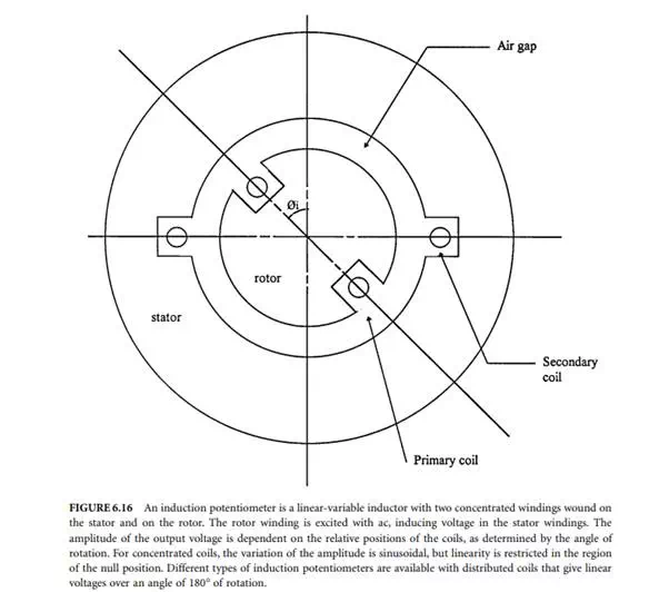
One version of a rotary type linear inductor is the induction potentiometer shown in Figure 6.16. Two concentrated windings are wound on the stator and rotor. The rotor winding is excited with an ac, thus inducing voltage in the stator windings. The amplitude of the output voltage is dependent on the mutual inductance between the two coils, where mutual inductance itself is dependent on the angle of rotation. For concentrated coil type induction potentiometers, the variation of the amplitude is sinusoidal, but linearity is restricted in the region of the null position. A linear distribution over an angle of 180° can be obtained by carefully designed distributed coils.
Standard commercial induction pots operate in a 50 to 400 Hz frequency range. They are small in size, from 1 cm to 6 cm, and their sensitivity can be on the order of 1 V/deg rotation. Although the ranges of induction pots are limited to less than 60° of rotation, it is possible to measure displacements in angles from 0° to full rotation by suitable arrangement of a number of induction pots. As in the case of most
inductive sensors, the output of an induction pot may need phase-sensitive demodulators and suitable filters. In many cases, additional dummy coils are used to improve linearity and accuracy.
Linear Variable-Differential Transformer (LVDT)
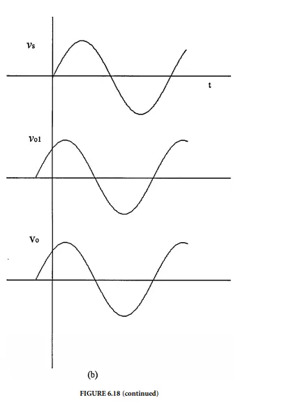
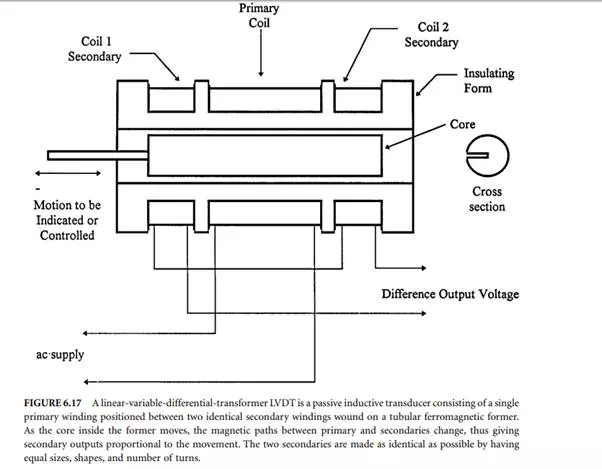
The linear variable-differential transformer, LVDT, is a passive inductive transducer finding many applications. It consists of a single primary winding positioned between two identical secondary windings wound on a tubular ferromagnetic former, as shown in Figure 6.17. The primary winding is energized by a high-frequency 50 Hz to 20 kHz ac voltage. The two secondary windings are made identical by having an equal number of turns and similar geometry. They are connected in series opposition so that the induced output voltages oppose each other. In many applications, the outputs are connected in opposing form, as shown in Figure 6.18(a). The output voltages of individual secondaries v1 and v2 at null position are illustrated in Figure 6.18(b). However, in opposing connection, any displacement in the core position x from the null point causes amplitude of the voltage output vo and the phase difference α to change. The output waveform vo in relation to core position is shown in Figure 6.18(c). When the core is positioned in the middle, there is
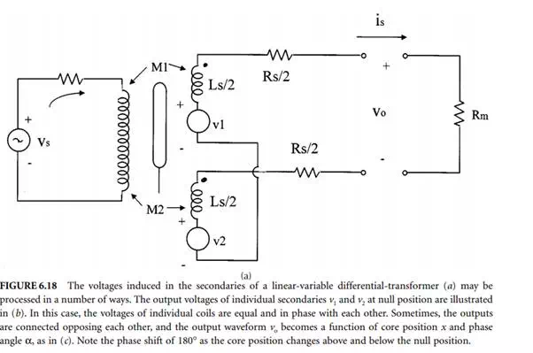
an equal coupling between the primary and secondary windings, thus giving a null point or reference point of the sensor. As long as the core remains near the center of the coil arrangement, output is very linear. The linear ranges of commercial differential transformers are clearly specified, and the devices are seldom used outside this linear range. The ferromagnetic core or plunger moves freely inside the former, thus altering the mutual inductance between the primary and secondaries. With the core in the center, or at the reference position, the induced emfs in the secondaries are equal; and since they oppose each other, the output voltage is zero. When the core moves, say to the left, from the center, more magnetic flux links with the left-hand coil than with the right-hand coil. The voltage induced in the left-hand coil is therefore larger than the induced voltage on the right-hand coil. The magnitude of the output voltage is then larger than at the null position and is equal to the difference between the two secondary voltages. The net output voltage is in phase with the voltage of the left-hand coil. The output of the device is then an indication of the displacement of the core. Similarly, movement in the opposite direction to the right from the centre reverses this effect, and the output voltage is now in phase with the emf of the right-hand coil.
For mathematical analysis of the operation of LVDTs, Figure 6.18(a) can be used. The voltages induced in the secondary coils are dependent on the mutual inductance between the primary and individual secondary coils. Assuming that there is no cross-coupling between the secondaries, the induced voltages may be written as:
where M1 and M2 are the mutual inductances between primary and secondary coils for a fixed core position; s is the Laplace operator; and ip is the primary current