Purpose
One needs an estimate of the uncertainty of test results to make informed decisions. Ideally, the uncertainty of a well-run experiment will be much less than the change or test result expected. In this way, it will be known, with high confidence, that the change or result observed is real or acceptable and not a result of the errors of the test or measurement process. The limits of those errors are estimated with uncertainty, and those error sources and their limit estimators, the uncertainties, may be grouped into classifications to ease their understanding.
Classifying Error and Uncertainty Sources
There are two classification systems in use. The final total uncertainty calculated at a confidence is identical no matter what classification system is used. The two classifications utilized are the ISO classifications and the engineering classifications. The former groups errors and their uncertainties by type, depending on whether or not there is data available to calculate the sample standard deviation for a particular error and its uncertainty. The latter classification groups errors and their uncertainties by their effect on the experiment or test. That is, the engineering classification groups errors and uncertainties by random and systematic types, with subscripts used to denote whether there are data to calculate a standard deviation or not for a particular error or uncertainty source. For this reason, engineering classification groups usually are more useful and recommended.
ISO Classifications
This error and uncertainty classification system is not recommended in this chapter, but will yield a total uncertainty in complete agreement with the recommended classification system — the engineering classification system. In this ISO system, errors and uncertainties are classified as Type A if there are data to calculate a sample standard deviation and Type B if there is not [4]. In the latter case, the sample standard deviation might be obtained from experience or manufacturer’s specifications, to name two examples.
The impact of multiple sources of error is estimated by root-sum-squaring their corresponding multiple uncertainties. The operating equations are Type A, data for the calculation of the standard deviation:
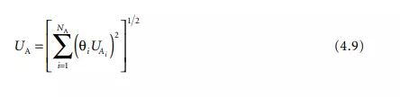
The uncertainty of each error source in units of that source, when multiplied by the sensitivity for that source, converts that uncertainty to result units. Then the effect of several error sources may be estimated by root-sum-squaring their uncertainties as they are now all in the same units. The sensitivities, θi , are obtained for a measurement result, R, which is a function of several parameters, Pi . The basic equations are
R = the measurement result

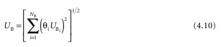

For these uncertainties, it is assumed that the UBi represent one standard deviation of the average for one uncertainty source with an assumed normal distribution. (They also represent one standard deviation as the square root of the “M” by which they are divided is one, that is, there is only one Type B error sampled from each of these distributions.) The degrees of freedom associated with this standard deviation (also standard deviation of the average) is infinity.
Note that θi , the sensitivity of the test or measurement result to the i th Type B uncertainty, is actually the change in the result, R, that would result from a change, of the size of the Type B uncertainty, in the i th input parameter used to calculate that result.
The degrees of freedom of the UA and the UBi are needed to compute the degrees of freedom of the combined total uncertainty. It is calculated with the Welch–Satterthwaite approximation. The general formula for degrees of freedom [5] is

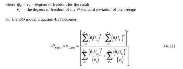
The degrees of freedom calculated with Equation 4.12 is often a fraction. This should be truncated to the next lower whole number to be conservative.
Note that in Equations 4.9, 4.10, and 4.12, NA and NB need not be equal. They are only the total number of parameters with uncertainty sources of Type A and B, respectively.
In computing a total uncertainty, the uncertainties noted by Equations 4.10 and 4.11 are combined. For the ISO model [3], this is calculated as:


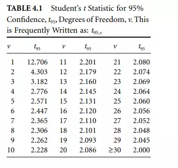
Student’s t is obtained from Table 4.1.
Note that alternative confidences are permissible. 95% is recommended by the ASME [6], but 99% or 99.7% or any other confidence is obtained by choosing the appropriate Student’s t. 95% confidence is, however, recommended for uncertainty analysis.
In all the above, the errors were assumed to be independent. Independent sources of error are those that have no relationship to each other. That is, an error in a measurement from one source cannot be used to predict the magnitude or direction of an error from the other, independent, error source. Non-independent error sources are related. That is, if it were possible to know the error in a measurement from one source, one could calculate or predict an error magnitude and direction from the other,
nonindependent error source. These are sometimes called dependent error sources. Their degree of dependence may be estimated with the linear correlation coefficient. If they are nonindependent, whether Type A or Type B, Equation 4.13 becomes [7]:

This ISO classification equation will yield the same total uncertainty as the engineering classification, but the ISO classification does not provide insight into how to improve an experiment’s or test’s uncertainty. That is, whether to possibly take more data because the random uncertainties are too high or calibrate better because the systematic uncertainties are too large. The engineering classification now presented is therefore the preferred approach.