Error: The Normal Distribution and the Uniform Distribution
Error is defined as the difference between the measured value and the true value of the measurand [1]. That is,
where
E = the measurement error
(measured) = the value obtained by a measurement
(true) = the true value of the measurand
It is only possible to estimate, with some confidence, the expected limits of error. The most common method for estimating those limits is to use the normal distribution [2]. It is

where
X = the input variable, here the value obtained by a measurement
µ = the average of the population of the X variable
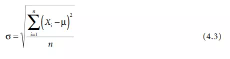
σ = the standard deviation of the population, expressed as:
where
Xi = the i th X measurement
n = the number of data points measured from the population
Typically, neither n, µ, nor σ are known.
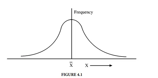
Figure 4.1 illustrates this distribution. Here, for an infinite population (N = ∞), the standard deviation, σ, would be used to estimate the expected limits of a particular error with some confidence. That is, the average, plus or minus 2σ divided by the square root of the number of data points, would contain the true average, µ, 95% of the time.
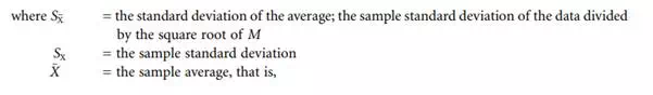
However, in test measurements, one typically cannot sample the entire population and must make do with a sample of N data points. The sample standard deviation, SX, is then used to estimate σX, the expected limits of a particular error. (That sample standard deviation divided by the square root of the number of data points is the starting point for the confidence interval estimate on µ.) For a large dataset (defined as having 30 or more degrees of freedom), plus or minus 2SX divided by the square root of the number of data points in the reported average, M, would contain the true average, µ, 95% of the time. That SX divided by the square root of the number of data points in the reported average is called the standard deviation of the average and is written as:
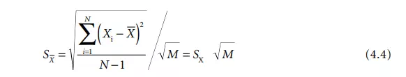
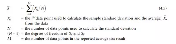
Note in Equation 4.4 that N does not necessarily equal M . It is possible to obtain SX from historical data with many degrees of freedom ([N – 1] greater than 30) and to run the test only M times. The test result, or average, would therefore be based on M measurements, and the standard deviation of the average would still be calculated with Equation 4.4. In that case, there would be two averages, – X. One – X would be from the historical data used to calculate the sample standard deviation, and the other – X, the average test result for M measurements.
Note that the sample standard deviation, SX, is simply

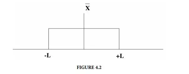
In some cases, a particular error distribution may be assumed or known to be a uniform or rectangular distribution, Figure 4.2, instead of a normal distribution. For those cases, the sample standard deviation of the data is calculated as:
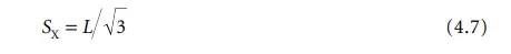
where L = the plus/minus limits of the uniform distribution for a particular error [3]. For those cases, the standard deviation of the average is written as:

Although the calculation of the sample standard deviation (or its estimation by some other process) is required for measurement uncertainty analysis, all the analytical work computing the measurement uncertainty uses only the standard deviation of the average for each error source.
Uncertainty (Accuracy)
Since the error for any particular error source is unknown and unknowable, its limits, at a given confidence, must be estimated. This estimate is called the uncertainty. Sometimes, the term accuracy is used to describe the quality of test data. This is the positive statement of the expected limits of the data’s errors. Uncertainty is the negative statement. Uncertainty is, however, unambiguous. Accuracy is sometimes ambiguous. (For example,: what is twice the accuracy of ±2%? ±1% or ±4%?) For this reason, this chapter will use the term uncertainty throughout to describe the quality of test data.