Output/Input Relationship

Instrument systems are usually built up from a serial linkage of distinguishable building blocks. The actual physical assembly may not appear to be so but it can be broken down into a representative diagram of connected blocks. Figure 3.4 shows the block diagram representation of a humidity sensor. The sensor is activated by an input physical parameter and provides an output signal to the next block that processes the signal into a more appropriate state.

A key generic entity is, therefore, the relationship between the input and output of the block. As was pointed out earlier, all signals have a time characteristic, so we must consider the behavior of a block in terms of both the static and dynamic states.

The behavior of the static regime alone and the combined static and dynamic regime can be found through use of an appropriate mathematical model of each block. The mathematical description of system responses is easy to set up and use if the elements all act as linear systems and where addition of signals can be carried out in a linear additive manner. If nonlinearity exists in elements, then it becomes considerably more difficult — perhaps even quite impractical — to provide an easy to follow mathematical explanation. Fortunately, general description of instrument systems responses can be usually be adequately covered using the linear treatment.

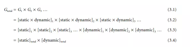
The output/input ratio of the whole cascaded chain of blocks 1, 2, 3, etc. is given as: [output/input]total = [output/input]1 × [output/input]2 × [output/input]3 …

The output/input ratio of a block that includes both the static and dynamic characteristics is called the transfer function and is given the symbol G.

 The equation for G can be written as two parts multiplied together. One expresses the static behavior of the block, that is, the value it has after all transient (time varying) effects have settled to their final state. The other part tells us how that value responds when the block is in its dynamic state. The static part is known as the transfer characteristic and is often all that is needed to be known for block description.

The static and dynamic response of the cascade of blocks is simply the multiplication of all individual blocks. As each block has its own part for the static and dynamic behavior, the cascade equations can be rearranged to separate the static from the dynamic parts and then by multiplying the static set and the dynamic set we get the overall response in the static and dynamic states. This is shown by the sequence of Equations 3.1 to 3.4.

An example will clarify this. A mercury-in-glass fever thermometer is placed in a patient’s mouth. The indication slowly rises along the glass tube to reach the final value, the body temperature of the person. The slow rise seen in the indication is due to the time it takes for the mercury to heat up and expand up the tube. The static sensitivity will be expressed as so many scale divisions per degree and is all that is of interest in this application. The dynamic characteristic will be a time varying function that settles to unity after the transient effects have settled. This is merely an annoyance in this application but has to be allowed by waiting long enough before taking a reading. The wrong value will be viewed if taken before the transient has settled.

At this stage, we will now consider only the nature of the static characteristics of a chain; dynamic response is examined later.

If a sensor is the first stage of the chain, the static value of the gain for that stage is called the sensitivity. Where a sensor is not at the input, it is called the amplification factor or gain. It can take a value less than unity where it is then called the attenuation.

Sometimes, the instantaneous value of the signal is rapidly changing, yet the measurement aspect part is static. This arises when using ac signals in some forms of instrumentation where the amplitude of the waveform, not its frequency, is of interest. Here, the static value is referred to as its steady state transfer characteristic.

Sensitivity may be found from a plot of the input and output signals, wherein it is the slope of the graph. Such a graph, see Figure 3.5, tells much about the static behavior of the block.

The intercept value on the y-axis is the offset value being the output when the input is set to zero. Offset is not usually a desired situation and is seen as an error quantity. Where it is deliberately set up, it is called the bias.

The range on the x-axis, from zero to a safe maximum for use, is called the range or span and is often expressed as the zone between the 0% and 100% points. The ratio of the span that the output will cover

for the related input range is known as the dynamic range. This can be a confusing term because it does not describe dynamic time behavior. It is particularly useful when describing the capability of such instruments as flow rate sensors — a simple orifice plate type may only be able to handle dynamic ranges of 3 to 4, whereas the laser Doppler method covers as much as 107 variation.

Drift

It is now necessary to consider a major problem of instrument performance called instrument drift. This is caused by variations taking place in the parts of the instrumentation over time. Prime sources occur as chemical structural changes and changing mechanical stresses. Drift is a complex phenomenon for which the observed effects are that the sensitivity and offset values vary. It also can alter the accuracy of the instrument differently at the various amplitudes of the signal present.

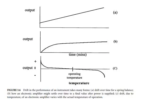
Detailed description of drift is not at all easy but it is possible to work satisfactorily with simplified values that give the average of a set of observations, this usually being quoted in a conservative manner. The first graph (a) in Figure 3.6 shows typical steady drift of a measuring spring component of a weighing balance. Figure 3.6(b) shows how an electronic amplifier might settle down after being turned on.

Drift is also caused by variations in environmental parameters such as temperature, pressure, and humidity that operate on the components. These are known as influence parameters. An example is the change of the resistance of an electrical resistor, this resistor forming the critical part of an electronic amplifier that sets its gain as its operating temperature changes.

Unfortunately, the observed effects of influence parameter induced drift often are the same as for time varying drift. Appropriate testing of blocks such as electronic amplifiers does allow the two to be separated to some extent. For example, altering only the temperature of the amplifier over a short period will quickly show its temperature dependence.

Drift due to influence parameters is graphed in much the same way as for time drift. Figure 3.6(c) shows the drift of an amplifier as temperature varies. Note that it depends significantly on the temperature of operation, implying that the best designs are built to operate at temperatures where the effect is minimum.

Careful consideration of the time and influence parameter causes of drift shows they are interrelated and often impossible to separate. Instrument designers are usually able to allow for these effects, but the cost of doing this rises sharply as the error level that can be tolerated is reduced.

Hysteresis and Backlash

Careful observation of the output/input relationship of a block will sometimes reveal different results as the signals vary in direction of the movement. Mechanical systems will often show a small difference in length as the direction of the applied force is reversed. The same effect arises as a magnetic field is reversed in a magnetic material. This characteristic is called hysteresis. Figure 3.7 is a generalized plot of the output/input relationship showing that a closed loop occurs. The effect usually gets smaller as the amplitude of successive excursions is reduced, this being one way to tolerate the effect. It is present in most materials. Special materials have been developed that exhibit low hysteresis for their application — transformer iron laminations and clock spring wire being examples.

Where this is caused by a mechanism that gives a sharp change, such as caused by the looseness of a joint in a mechanical joint, it is easy to detect and is known as backlash.

Saturation

So far, the discussion has been limited to signal levels that lie within acceptable ranges of amplitude. Real system blocks will sometimes have input signal levels that are larger than allowed. Here, the dominant errors that arise — saturation and crossover distortion — are investigated.

As mentioned above, the information bearing property of the signal can be carried as the instantaneous value of the signal or be carried as some characteristic of a rapidly varying ac signal. If the signal form is not amplified faithfully, the output will not have the same linearity and characteristics.

The gain of a block will usually fall off with increasing size of signal amplitude. A varying amplitude input signal, such as the steadily rising linear signal shown in Figure 3.8, will be amplified differently according to the gain/amplitude curve of the block. In uncompensated electronic amplifiers, the larger amplitudes are usually less amplified than at the median points.

At very low levels of input signal, two unwanted effects may arise. The first is that small signals are often amplified more than at the median levels. The second error characteristic arises in electronic amplifiers because the semiconductor elements possess a dead-zone in which no output occurs until a small threshold is exceeded. This effect causes crossover distortion in amplifiers.

If the signal is an ac waveform, see Figure 3.9, then the different levels of a cycle of the signal may not all be amplified equally. Figure 3.9(a) shows what occurs because the basic electronic amplifying elements are only able to amplify one polarity of signal. The signal is said to be rectified. Figure 3.9(b) shows the effect when the signal is too large, and the top is not amplified. This is called saturation or clipping. (As with many physical effects, this effect is sometimes deliberately invoked in circuitry, an example being where it is used as a simple means to convert sine-waveform signals into a square waveform.) Crossover distortion is evident in Figure 3.9(c) as the signal passes from negative to positive polarity.

Where input signals are small, such as in sensitive sensor use, the form of analysis called small signal behavior is needed to reveal distortions. If the signals are comparatively large, as for digital signal considerations, a large signal analysis is used. Design difficulties arise when signals cover a wide dynamic range because it is not easy to allow for all of the various effects in a single design.