Before we can begin to develop an understanding of the static and time changing characteristics of measurements, it is necessary to build a framework for understanding the process involved, setting down the main words used to describe concepts as we progress.
Measurement is the process by which relevant information about a system of interest is interpreted using the human thinking ability to define what is believed to be the new knowledge gained. This information may be obtained for purposes of controlling the behaviour of the system (as in engineering applications) or for learning more about it (as in scientific investigations). The basic entity needed to develop the knowledge is called data, and it is obtained with physical assemblies known as sensors that are used to observe or sense system variables. The terms information and knowledge tend to be used interchangeably to describe the entity resulting after data from one or more sensors have been processed to give more meaningful understanding. The individual variables being sensed are called measurands.
The most obvious way to make observations is to use the human senses of seeing, feeling, and hearing. This is often quite adequate or may be the only means possible. In many cases, however, sensors are used that have been devised by man to enhance or replace our natural sensors. The number and variety of sensors is very large indeed. Examples of man-made sensors are those used to measure temperature, pressure, or length. The process of sensing is often called transduction, being made with transducers. These man-made sensor assemblies, when coupled with the means to process the data into knowledge, are generally known as (measuring) instrumentation.
The degree of perfection of a measurement can only be determined if the goal of the measurement can be defined without error. Furthermore, instrumentation cannot be made to operate perfectly. Because of these two reasons alone, measuring instrumentation cannot give ideal sensing performance and it must be selected to suit the allowable error in a given situation.
Measurement is a process of mapping actually occurring variables into equivalent values. Deviations from perfect measurement mappings are called errors: what we get as the result of measurement is not exactly what is being measured. A certain amount of error is allowable provided it is below the level of uncertainty we can accept in a given situation. As an example, consider two different needs to measure the measurand, time. The uncertainty to which we must measure it for daily purposes of attending a meeting is around a 1 min in 24 h. In orbiting satellite control, the time uncertainty needed must be as small as milliseconds in years. Instrumentation used for the former case costs a few dollars and is the watch we wear; the latter instrumentation costs thousands of dollars and is the size of a suitcase.
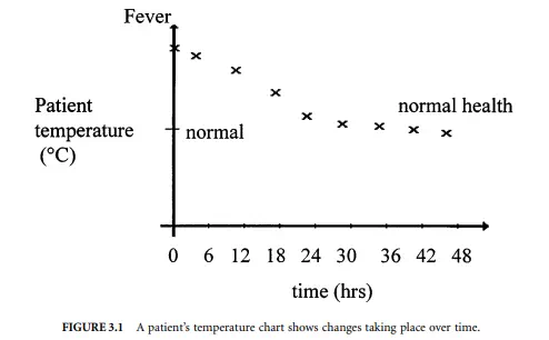
We often record measurand values as though they are constant entities, but they usually change in value as time passes. These “dynamic” variations will occur either as changes in the measurand itself or where the measuring instrumentation takes time to follow the changes in the measurand — in which case it may introduce unacceptable error.
For example, when a fever thermometer is used to measure a person’s body temperature, we are looking to see if the person is at the normally expected value and, if it is not, to then look for changes over time as an indicator of his or her health. Figure 3.1 shows a chart of a patient’s temperature. Obviously, if the thermometer gives errors in its use, wrong conclusions could be drawn. It could be in error due to incorrect calibration of the thermometer or because no allowance for the dynamic response of the thermometer itself was made.
Instrumentation, therefore, will only give adequately correct information if we understand the static and dynamic characteristics of both the measurand and the instrumentation. This, in turn, allows us to then decide if the error arising is small enough to accept.
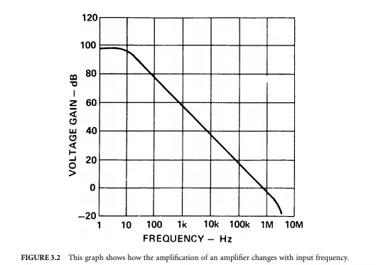
As an example, consider the electronic signal amplifier in a sound system. It will be commonly quoted as having an amplification constant after feedback if applied to the basic amplifier of, say, 10. The actual amplification value is dependent on the frequency of the input signal, usually falling off as the frequency increases. The frequency response of the basic amplifier, before it is configured with feedback that markedly alters the response and lowers the amplification to get a stable operation, is shown as a graph of amplification gain versus input frequency. An example of the open loop gain of the basic amplifier is given in Figure 3.2. This lack of uniform gain over the frequency range results in error — the sound output is not a true enough representation of the input.
Before we can delve more deeply into the static and dynamic characteristics of instrumentation, it is necessary to understand the difference in meaning between several basic terms used to describe the results of a measurement activity.
The correct terms to use are set down in documents called standards. Several standardized metrology terminologies exist but they are not consistent. It will be found that books on instrumentation and statements of instrument performance often use terms in different ways. Users of measurement information need to be constantly diligent in making sure that the statements made are interpreted correctly.
The three companion concepts about a measurement that need to be well understood are its discrimination, its precision, and its accuracy. These are too often used interchangeably — which is quite wrong to do because they cover quite different concepts, as will now be explained.
When making a measurement, the smallest increment that can be discerned is called the discrimination. (Although now officially declared as wrong to use, the term resolution still finds its way into books and reports as meaning discrimination.) The discrimination of a measurement is important to know because it tells if the sensing process is able to sense fine enough changes of the measurand.
Even if the discrimination is satisfactory, the value obtained from a repeated measurement will rarely give exactly the same value each time the same measurement is made under conditions of constant value of measurand. This is because errors arise in real systems. The spread of values obtained indicates the precision of the set of the measurements. The word precision is not a word describing a quality of the measurement and is incorrectly used as such. Two terms that should be used here are: repeatability, which describes the variation for a set of measurements made in a very short period; and the reproducibility, which is the same concept but now used for measurements made over a long period. As these terms describe the outcome of a set of values, there is need to be able to quote a single value to describe the overall result of the set. This is done using statistical methods that provide for calculation of the “mean value” of the set and the associated spread of values, called its variance.
The accuracy of a measurement is covered in more depth elsewhere so only an introduction to it is required here. Accuracy is the closeness of a measurement to the value defined to be the true value. This
concept will become clearer when the following illustrative example is studied for it brings together the three terms into a single perspective of a typical measurement.
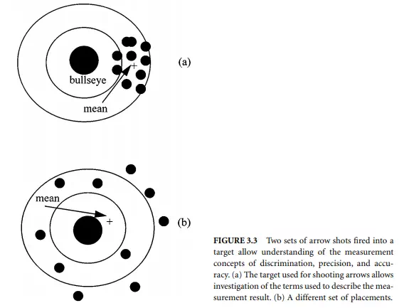
Consider then the situation of scoring an archer shooting arrows into a target as shown in Figure 3.3(a). The target has a central point — the bulls-eye. The objective for a perfect result is to get all arrows into the bulls-eye. The rings around the bulls-eye allow us to set up numeric measures of less-perfect shooting performance.
Discrimination is the distance at which we can just distinguish (i.e., discriminate) the placement of one arrow from another when they are very close. For an arrow, it is the thickness of the hole that decides the discrimination. Two close-by positions of the two arrows in Figure 3.3(a) cannot be separated easily. Use of thinner arrows would allow finer detail to be decided.
Repeatability is determined by measuring the spread of values of a set of arrows fired into the target over a short period. The smaller the spread, the more precise is the shooter. The shooter in Figure 3.3(a) is more precise than the shooter in Figure 3.3(b).
If the shooter returned to shoot each day over a long period, the results may not be the same each time for a shoot made over a short period. The mean and variance of the values are now called the reproducibility of the archer’s performance.
Accuracy remains to be explained. This number describes how well the mean (the average) value of the shots sits with respect to the bulls-eye position. The set in Figure 3.3(b) is more accurate than the set in Figure 3.3(a) because the mean is nearer the bulls-eye (but less precise!).
At first sight, it might seem that the three concepts of discrimination, precision, and accuracy have a strict relationship in that a better measurement is always that with all three aspects made as high as is affordable. This is not so. They need to be set up to suit the needs of the application.
We are now in a position to explore the commonly met terms used to describe aspects of the static and the dynamic performance of measuring instrumentation.