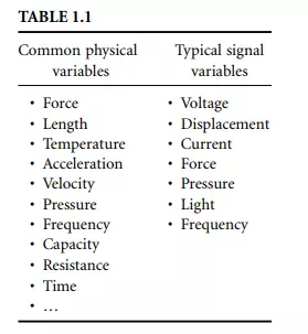
Figure 1.1 presents a generalized model of a simple instrument. The physical process to be measured is in the left of the figure and the measurand is represented by an observable physical variable X. Note that the observable variable X need not necessarily be the measurand but simply related to the measurand in some known way. For example, the mass of an object is often measured by the process of weighing, where the measurand is the mass but the physical measurement variable is the downward force the mass exerts in the Earth’s gravitational field. There are many possible physical measurement variables. A few are shown in Table 1.1.

The key functional element of the instrument model shown in Figure 1.1 is the sensor, which has the function of converting the physical variable input into a signal variable output. Signal variables have the property that they can be manipulated in a transmission system, such as an electrical or mechanical circuit. Because of this property, the signal variable can be transmitted to an output or recording device that can be remote from the sensor. In electrical circuits, voltage is a common signal variable. In mechanical systems, displacement or force are commonly used as signal variables. Other examples of signal variable are shown in Table 1.1. The signal output from the sensor can be displayed, recorded, or used as an input signal to some secondary device or system. In a basic instrument, the signal is transmitted to a display or recording device where the measurement can be read by a human observer. The observed output is the measurement M. There are many types of display devices, ranging from simple scales and dial gages to sophisticated computer display systems. The signal can also be used directly by some larger

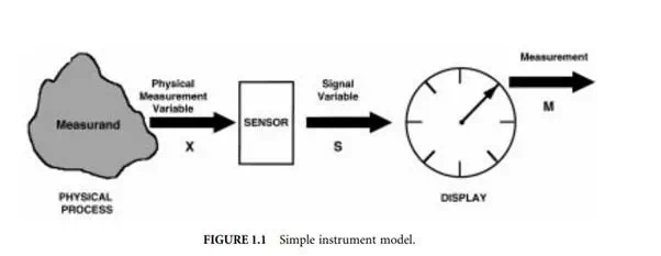
system of which the instrument is a part. For example, the output signal of the sensor may be used as the input signal of a closed loop control system.

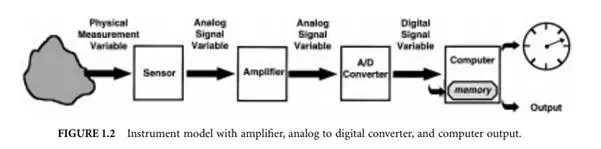
If the signal output from the sensor is small, it is sometimes necessary to amplify the output shown in Figure 1.2. The amplified output can then be transmitted to the display device or recorded, depending on the particular measurement application. In many cases it is necessary for the instrument to provide a digital signal output so that it can interface with a computer-based data acquisition or communications system. If the sensor does not inherently provide a digital output, then the analog output of the sensor is converted by an analog to digital converter (ADC) as shown in Figure 1.2. The digital signal is typically sent to a computer processor that can display, store, or transmit the data as output to some other system, which will use the measurement.

Passive and Active Sensors

As discussed above, sensors convert physical variables to signal variables. Sensors are often transducers in that they are devices that convert input energy of one form into output energy of another form. Sensors

can be categorized into two broad classes depending on how they interact with the environment they are measuring. Passive sensors do not add energy as part of the measurement process but may remove energy in their operation. One example of a passive sensor is a thermocouple, which converts a physical temperature into a voltage signal. In this case, the temperature gradient in the environment generates a thermoelectric voltage that becomes the signal variable. Another passive transducer is a pressure gage where the pressure being measured exerts a force on a mechanical system (diaphragm, aneroid or Borden pressure gage) that converts the pressure force into a displacement, which can be used as a signal variable. For example, the displacement of the diaphragm can be transmitted through a mechanical gearing system to the displacement of an indicating needle on the display of the gage.

Active sensors add energy to the measurement environment as part of the measurement process. An example of an active sensor is a radar or sonar system, where the distance to some object is measured by actively sending out a radio (radar) or acoustic (sonar) wave to reflect off of some object and measure its range from the sensor.

Calibration

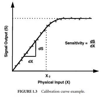
The relationship between the physical measurement variable input and the signal variable (output) for a specific sensor is known as the calibration of the sensor. Typically, a sensor (or an entire instrument system) is calibrated by providing a known physical input to the system and recording the output. The data are plotted on a calibration curve such as the example shown in Figure 1.3. In this example, the sensor has a linear response for values of the physical input less than X0. The sensitivity of the device is determined by the slope of the calibration curve. In this example, for values of the physical input greater than X0, the calibration curve becomes less sensitive until it reaches a limiting value of the output signal. This behaviour is referred to as saturation, and the sensor cannot be used for measurements greater than its saturation value. In some cases, the sensor will not respond to very small values of the physical input variable. The difference between the smallest and largest physical inputs that can reliably be measured by an instrument determines the dynamic range of the device.

Modifying and Interfering Inputs

In some cases, the sensor output will be influenced by physical variables other than the intended measurand. In Figure 1.4, X is the intended measurand, Y is an interfering input, and Z is a modifying input. The interfering input Y causes the sensor to respond in the same manner as the linear superposition of Y and the intended measurand X. The measured signal output is therefore a combination of X and Y,

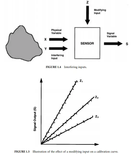
with Y interfering with the intended measurand X. An example of an interfering input would be a structural vibration within a force measurement system.

Modifying inputs changes the behaviour of the sensor or measurement system, thereby modifying the input/output relationship and calibration of the device. This is shown schematically in Figure 1.5. For various values of Z in Figure 1.5, the slope of the calibration curve changes. Consequently, changing Z will result in a change of the apparent measurement even if the physical input variable X remains constant. A common example of a modifying input is temperature; it is for this reason that many devices are calibrated at specified temperatures.

Accuracy and Error

The accuracy of an instrument is defined as the difference between the true value of the measurand and the measured value indicated by the instrument. Typically, the true value is defined in reference to some absolute or agreed upon standard. For any particular measurement there will be some error due to

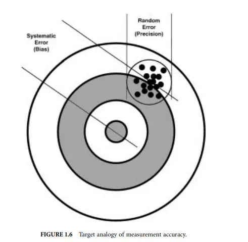
systematic (bias) and random (noise) error sources. The combination of systematic and random error can be visualized by considering the analogy of the target shown in Figure 1.6. The total error in each shot results from both systematic and random errors. The systematic (bias) error results in the grouping of shots being offset from the bulls eye (presumably a misalignment of the gunsight or wind). The size of the grouping is determined by random error sources and is a measure of the precision of the shooting.