INTRODUCTION

• The .selection of most suitable transducer from commercially available instruments is very important in designing an Instrumentation system.

• For the proper selection of transducer, knowledge of the performance characteristics ·of them are essential.

• The performance characteristics can be classified into two namely

(i) Static characteristics

(ii) Dynamic characteristics

·         Static characteristics are a set of performance criteria that give a meaningful description of the quality of measurement without becoming concerned with dynamic descriptions involving differential equations.

·         Dynamic characteristics describe the quality of measurement when the measured quantities vary rapidly with time. Here the dynamic relations between the instrument input and output must be examined, generally by the use of differential equations.

STATIC CHARACTERISTICS AND STATIC CALIBRATION

• The most important static characteristics of a transducer are

1.      Static sensitivity

2.      Linearity

3.       Precision / Accuracy

4.      ResoIution

5.      Hysteresis

6.      Range and span

7.      Input impedance and loading effect.

Staticcalibration

All these static characteristics are obtained by one form or another of the process of static calibration.  In general, static calibration refers to a situation in which all inputs

except the desired one are kept at some constant values.  The desired input is varied over some range in steps and the output values are noted.

The input – output relationship thus developed is called the static calibration valid under the stated constant conditions of all the other inputs.

Static sensitivity

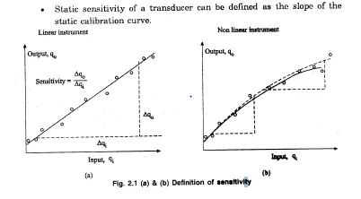
• If the curve is a straight line for a linear instrument, the sensitivity will vary with the input value, as shown in fig. (2.1) a.

•. If the curve is not a straight line for a non-linear instrument, the sensitivity will vary with the input value, as shown in fig. (2.1) b. .Hence the sensitivity should-be taken depending on the operating point.

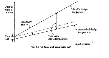
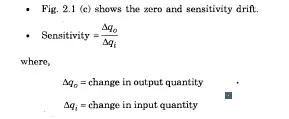
• The sensitivity is expressed in output unit / input unit. Zero and Sensitivity drift

• When the sensitivity of instrument to’ its desired input .is concerned, its sensitivity to interfering and/or modifying inputs is also to be .considered.

• For example, consider temperature as an input to the pressure gauge.

• Temperature can cause a relative expansion and contraction that will result in’ a change in output reading eveJ? though the pressure has not changed. Here, the temperature is. an .interfering input. This effect is called a zero drift.

• Also, temperature can alter the modulus 6felasticity of the’ pressure-gauge spring, thereby affecting the pressure sensitivity. Here, it is a” modifyin.g input. This effect is a’ sensitivity drift or scale-factor drift.

Linearity

•The calibration curve of a transducer may not be linear in many cases.

• If it is so, the transducer may still be highly accurate.

• However, linear behaviour is most desirable in many applications.

• The conversion from a scale reading to the corresponding measured value of input quantity is most convenient if it is to be multiplied by a fixed constant rather than looking into a calibration chart or a graph.

• Linearity is a measure of the maximum deviation of the plotted transducer response from a specified straight line.

• To select a straight line for a plotted calibration curve there are a number of ways. Some of them are

1. The straight line connecting the calibration point at zero input to that at full-scale input.

2. The straight line may be drawn through as many calibration points as possible.

3. The straight line may be determined by the least squares fit method mathematically. The input-output relationship of a transducer is generally given by the equation

y =ao +alx +a~2,+ a3x3 + …. +anxn … (2.1)

The best-fit straight line is mathematically determined by evaluating the deviation of the response curve from the straight line at a number of calibration points and choosing the one that gives the minimum of the sum of the squares of the deviations.

• This procedure is described as least squares fit.