Compared to their analog counterparts, digital filters offer outstanding performance and flexibility. Designing digital filters can seem a daunting task, however, because of its seemingly endless range of implementation choices. The wide range of digital signal processing (DSP) design tools available can handle many of the details. What you need is a good handle on the basics of filter design to get the tools jump-started. The place to start is by knowing type of information a signal contains. Information typically comes from one of two domains. It may lie in the frequency domain, where the spectral content of the signal is of interest. Information may also lie in the time domain, where the amplitude and phase of the signal is of interest. The term time domain is somewhat misleading, however, in that not all such signals relate to time. For example, a single sample from each element in an array of strain sensors on an aircraft ring yields a “signal” that can be processed using time-domain filters.

Reverse Filtering

One of the drawbacks to recursive (IIR) filters is that their phase characteristics are non-linear. For some kinds of signals, such as normal audio, this is not a problem. The phase in those signals is random to begin with. Other types of frequency-domain signals, however, need a linear phase relationship in order to preserve the desired information.  You can solve this problem for IIR filters at a cost of doubling the execution time and complexity. You use a technique called reverse filtering to correct the phase errors introduced in the original filter. In essence, you run time backwards.   This sounds like impossibility, but in the digital world it is quite simple. Since you already have all of the past data values stored from the initial filter calculation, you simply run the filter using later values instead of prior values. The difference equation becomes: 

y[n]=a0x[n]+a1x[n+1]+…+b1y[n+1]+b2y[n+2]+…

This does add a delay. You have to wait as many samples as the filter order before you can calculate the first output value. The result of normal filtering followed by reverse filtering, however, is a signal with zero phase delay.

A second consideration is the type of filter implementation you want to use. As described in Digital Filters: an Introduction, by Iain A. Robin, digital filters come in two types: convolution and recursive. Convolution filters, also called Finite Impulse Response (FIR) filters, have the attribute of exhibiting no phase distortion. There is a delay, of course, but all incoming samples receive the same treatment so that signal phase relationships are preserved. High-order FIR filters can be readily implemented and will achieve extremely high performance, although they may require many resources to implement. Recursive filters, also called Infinite Impulse Response (IIR) filters, can be implemented with far fewer resources than a corresponding FIR. This makes them both easier to implement and an order of magnitude faster in execution as a DSP algorithm. IIRs do, however, exhibit a non-linear phase response unless specifically designed for zero phase. They also suffer from performance limitations because finite word length arithmetic restricts the maximum IIR filter order that can be implemented.

Step Response

With these two considerations in mind, you can begin evaluating filter characteristics against your application. Filters are most easily understood from either their step response or their frequency response. The step response, important in time domain applications, is the filter’s output given an abrupt change in the input signal as illustrated in Figure 1. Step responses have three important parameters: risetime, overshoot, and phase linearity.

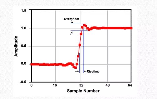Figure 1:  Step response is the filter’s output given an abrupt change in the input signal.

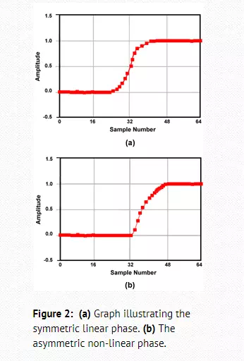
Risetime is the number of output samples between 10% of the output change and 90% of the change. Because time domain filters are typically used to help identify events in the signal (such as a bit boundary), the faster the risetime the better the filter. Overshoot is a filter-generated distortion of the time domain information, which shows up as ripples at the edges of the output step. It is a distortion that should be eliminated if possible because it could mask critical system performance information. When the filter has overshoot, it becomes impossible to determine whether the signal is being distorted by the system that generates it, or by the filter. Phase linearity for step responses refers to the symmetry of the step response above and below the 50% mark. As shown in Figure 2, a linear phase is symmetric about the halfway point while asymmetry occurs with non-linear phase. Linear phase ensures that rising edges of the filtered signal look like falling edges.

Frequency Response

Frequency response is important in frequency domain applications. The response, shown in Figure 3, has a passband and a stopband to select the frequencies of interest and discard all others. The boundary between the passband and stopband is the transition band, which occurs around the filter’s cutoff frequency. The width of this transition band is the filter’s roll-off, which is one of the important parameters of a frequency domain filter. In general, a faster roll-off is better.

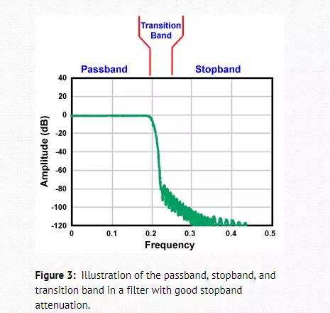
Passband ripple is a second important parameter. It represents a distortion of signals occurring in the passband. Ideally, there should be no passband ripple so that the desired signals pass through unaltered. The ideal filter also completely eliminates signals in the stopband. In practice, however, some energy in stopband frequencies will pass through. The amount by which the filter reduces the stopband signal is the filter’s stopband attenuation, the third important time domain filter parameter.

There are four common types of frequency-domain filters:

·         Low-pass

·         High-pass

·         Band-pass

·         Band-reject.

All of them can be evaluated using the three parameters.

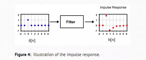
Impulse Response

Although the step and frequency responses are important for evaluating a digital filter, there is a third type of response that is important in implementing the filter: the impulse response. The impulse response, illustrated in Figure 4, is the filter’s output upon receiving a signal that has only one non-zero sample, called a delta function (d[n]). The most straightforward way of implementing a digital filter is to create an FIR that convolves an impulse response h[n] (also called the filter kernel) with the input signal x[n] using:

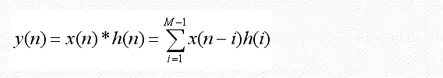
where M is the number of points used to express the filter kernel.

Each of the three responses contains complete information about the filter, so knowing one gives you the other two. The step response is the discrete integration of the impulse response. The frequency response comes from the discrete Fourier transform (DFT) of the impulse response. A filter design can, therefore, begin with a response description in any of the forms.

These designs don’t necessarily have to be complex. One of the most useful FIR time-domain filters, the moving average filter, is ideal for removing random (white) noise from a time-domain signal such as a serial bit stream. The transfer function of a moving average of length M is

This is easily implemented in an FIR simply by storing the last M samples and adding them together. For an IIR the thing to realize is that the moving average takes in one new sample and drops the oldest sample each sample period, so

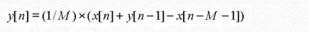
The moving average filter reduces random noise in a signal by a factor square root M. So, a 100-point filter would reduce noise by a factor of 10. Unfortunately, the step response of a moving average filter has a risetime that increases with the M, which is undesirable. As it turns out, however, it has the fastest risetime for a given level of noise reduction of any time-domain filter. No matter what, then, you’ll have to compromise between noise reduction and risetime.

The moving average is an excellent smoothing filter, but its frequency roll-off is slow and its stopband attenuation is ghastly, making it a terrible low-pass filter. This is typical; a digital filter can be optimized for time domain performance or frequency domain performance, but not both.

Windowed Sinc Low-Pass Filter

An appropriate FIR filter for frequency domain is the windowed-sinc filter. This low-pass filter uses the sinc function (sin(x)/x) for its filter kernel, where the value of the kernel components is given by:

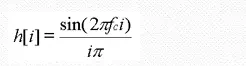
Where f_c is the desired cutoff frequency expressed as a fraction of the sampling frequency. If the filter kernel had an infinite number of points the result would be an ideal low-pass filter with no passband ripple, infinite attenuation in the stopband, and an infinitesimal transition band.

Unfortunately, an infinite number of points is not a good size for a filter kernel. One simple solution is to limit the number of points in the kernel by choosing M+1 points around the center of symmetry and ignoring all the rest. This, in effect, sets the remaining values to zero.

Choosing a Window

The value of M sets the filter’s roll-off characteristics. With an infinite number of points, the roll-off is infinitely steep: the output goes from one to zero in a single sample. With a finite number, the transition band bandwidth is given by:

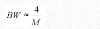
Where the bandwidth is expressed as a fraction of the sampling frequency and must be between 0 and 0.5.

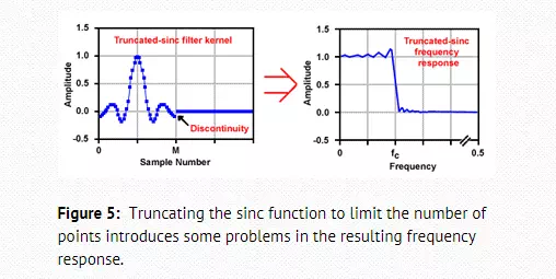
Simply truncating the sinc function to limit the number of points introduces some problems in the resulting frequency response, however, as shown in Figure 5. The discontinuity in the impulse response causes ripple in the passband and reduces stopband attenuation. To solve that problem, the windowed-sinc filter uses a filter kernel that is the product of the sinc function and a smoothly tapered window function.

A variety of such window functions are possible, but two of the most useful are the Blackman and Hamming windows. Both are mathematically derived functions that bring the function and its first derivative to zero at the endpoints, resulting in a much smoother frequency response. The Blackman window has the better stopband attenuation of the two: -74 dB versus -53 dB for the Hamming window. The Hamming window, on the other hand, has about a 20% faster roll-off.

Forming Other Filters

With a good low-pass filter in hand, the other common types of frequency-domain filters are easy to obtain. You can, for instance, design a high-pass filter directly from the impulse response of a low-pass filter. There are two ways of handling this conversion: spectral inversion and spectral reversal.

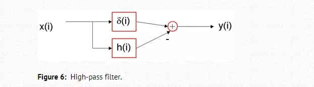
Spectral inversion gives a frequency response that is an inversion (flipped top to bottom) of the corresponding low-pass filter. You calculate the coefficients by reversing the sign of all kernel components except the center one. The new center component is simply (1- the old center component). Figure 6 shows schematically how this works. The high-pass filter output is simply the low-pass filter’s output subtracted from an all-pass filter (the delta function).

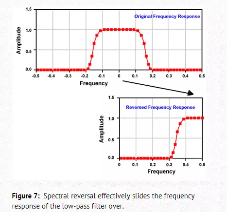
Spectral reversal is less intuitive. In this approach, you change the sign of alternate kernel components. In effect, you have multiplied the filter kernel by a sinusoid with a frequency one half the sampling rate, which shifts the filter’s frequency response by f_s/2. This results in a frequency response that is “flipped” left to right. The approach works because the frequency response of any digital filter is symmetric around zero frequency and repeats at the sampling frequency. As shown in Figure 7, spectral reversal effectively slides the frequency response of the low-pass filter over.

With both low-pass and high-pass filters in hand, it is easy to see how to build a band-reject filter. Simply add the results of the two filters together to get the total response. The band-reject kernel is the vector sum of the two filter kernels.

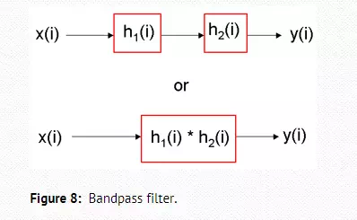
You can use spectral inversion or spectral reversal on the band-reject filter to obtain a band-pass filter. You can also create a band-pass filter by cascading the low-and high-pass filters, as shown in Figure 8. If you need a single filter with the same characteristics, you have to convolve the kernels of the two filters to generate the band-pass filter kernel.

The Z-Transform

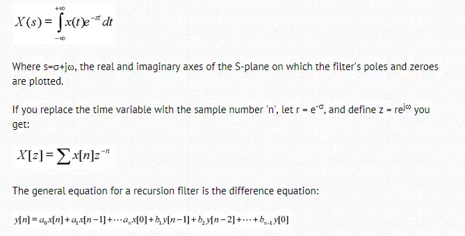
These simple FIR filters can meet many modest application needs. They can be inefficient to implement, however, and an IIR (recursive) filter may be what you need instead. To create an IIR, you will have to use the Z-transform. The Z-transform is the digital equivalent of the Laplace transform that analog filter designers use:

Low-Pass IIR

You don’t need all this complexity, however. If all you want is a simple low-pass filter, equivalent to an RC circuit, you can use the single-pole version. In this case, a₀ = 1-x and b₁ = x. All other terms are zero. The parameter ‘x’ determines the amount of decay between samples and can be found from x=e^-1/d where ‘d’ is the number of samples needed for a step input to decay to 36.8% of its final value. This is equivalent to the RC time constant of the corresponding analog circuit.

Similarly, the equivalent to a high-pass RC circuit has the values a₀ = (1+x)/2, a₁ = -(1+x)/2, and b₀ = x. An alternative way of picking x is to use x = e^-2pfc. Here fc is the 3dB cutoff frequency, expressed as a fraction of the sampling frequency with a value between 0 and 0.5.

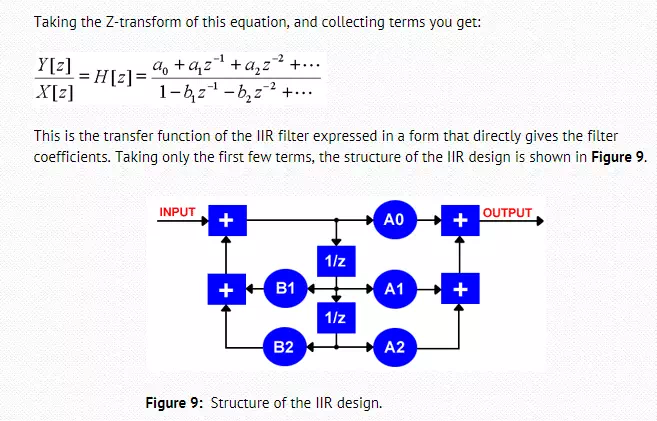
If you need to move beyond these simple filters, your best bet is to use some of the excellent DSP design software available. If you want to try your hand without a special tool, you can design an arbitrary digital filter as you would an analog filter. First, determine the analog poles and zeroes in the S-plane, then use the substitutions from the derivation of the Z-transform. This gives you the poles and zeroes in the Z-plane, allowing you to write the transfer function as:

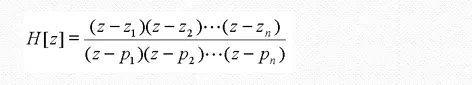
Once you know the poles and zeroes you want you can plug them in, do a little algebraic manipulation to put the equation in the other form, and read off the filter coefficients.

Of course, it doesn’t end there. Finite word length arithmetic and round off errors may shift the effective poles and zeroes off far enough to make the filter unstable. Only careful testing and tweaking will allow you to develop a custom filter that works as intended.