Systematic error (also called systematic bias) is consistent, repeatable error associated with faulty equipment or a flawed experiment design. These errors are usually caused by measuring instruments that are incorrectly calibrated or are used incorrectly. However, they can creep into your experiment from many sources, including:

·         A worn out instrument. For example, a plastic tape measure becomes slightly stretched over the years, resulting in measurements that are slightly too high.

·         An incorrectly calibrated or tared instrument, like a scale that doesn’t read zero when nothing is on it.

·         A person consistently takes an incorrect measurement. For example, they might think the 3/4″ mark on a ruler is the 2/3″ mark.

System Disturbance Due to Measurement

About system disturbance due to measurement

Disturbance of the measured system by the act of measurement is one source of systematic error. If we were to start with a beaker of hot water and wished to measure its temperature with a mercury-in-glass thermometer, then we would take the thermometer, which would be initially at room temperature, and plunge it into the water. In so doing, we would be introducing a relatively cold mass (the thermometer) into the hot water and a heat transfer would take place between the water and the thermometer. This heat transfer would lower the temperature of the water. Whilst in this case the reduction in temperature would be so small as to be undetectable by the limited measurement resolution of such a thermometer, the effect is finite and clearly establishes the principle that, in nearly all measurement situations, the process of measurement disturbs the system and alters the values of the physical quantities being measured.

Another example is that of measuring car tire pressures with the type of pressure gauge commonly obtainable from car accessory shops. Measurement is made by pushing one end of the pressure gauge on to the valve of the tire and reading the displacement of the other end of the gauge against a scale. As the gauge is used, a quantity of air flows from the tire into the gauge. This air does not subsequently flow back into the tire after measurement, and so the tire has been disturbed and the air pressure inside it has been permanently reduced.  Thus, as a general rule, the process of measurement always disturbs the system being measured. The magnitude of the disturbance varies from one measurement system to the next and is affected particularly by the type of instrument used for measurement. Ways of minimizing the disturbance of measured systems are an important consideration in instrument design. A prerequisite for this, however, is an accurate understanding of the mechanisms of system disturbance.

Measurements in electric circuits

In analysing system disturbance during measurements in electric circuits, Thevenin’s ´ theorem (see Appendix 3) is often of great assistance. For instance, consider the circuit shown in Figure 3.1(a) in which the voltage across resistor R5 is to be measured by a voltmeter with resistance Rm. Here, Rm acts as a shunt resistance across R5, decreasing the resistance between points AB and so disturbing the circuit. Therefore, the voltage Em measured by the meter is not the value of the voltage E0 that existed prior to measurement. The extent of the disturbance can be assessed by calculating the opencircuit voltage E0 and comparing it with Em.

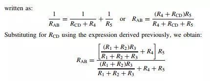
Thevenin’s theorem allows the circuit of Figure 3.1(a) comprising two voltage ´ sources and five resistors to be replaced by an equivalent circuit containing a single resistance and one voltage source, as shown in Figure 3.1(b). For the purpose of defining the equivalent single resistance of a circuit by Thevenin’s theorem, all voltage ´ sources are represented just by their internal resistance, which can be approximated to zero, as shown in Figure 3.1(c). Analysis proceeds by calculating the equivalent resistances of sections of the circuit and building these up until the required equivalent resistance of the whole of the circuit is obtained. Starting at C and D, the circuit to the left of C and D consists of a series pair of resistances (R1 and R2) in parallel with R3, and the equivalent resistance can be written as:

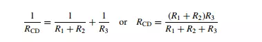
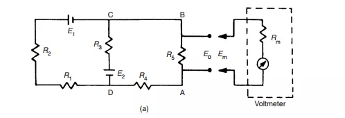
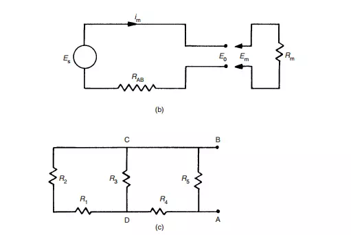
Fig. 3.1 Analysis of circuit loading: (a) a circuit in which the voltage across R5 is to be measured; (b) equivalent circuit by Th´evenin’s theorem; (c) the circuit used to find the equivalent single resistance RAB.

Errors during the measurement process

Defining I as the current flowing in the circuit when the measuring instrument is connected to it, we can write:

and the voltage measured by the meter is then given by:

In the absence of the measuring instrument and its resistance Rm, the voltage across AB would be the equivalent circuit voltage source whose value is E0. The effect of measurement is therefore to reduce the voltage across AB by the ratio given by:

It is thus obvious that as Rm gets larger, the ratio Em/E0 gets closer to unity, showing that the design strategy should be to make Rm as high as possible to minimize disturbance of the measured system. (Note that we did not calculate the value of E0, since this is not required in quantifying the effect of Rm.)

Errors due to environmental inputs

An environmental input is defined as an apparently real input to a measurement system that is actually caused by a change in the environmental conditions surrounding the measurement system. The fact that the static and dynamic characteristics specified for measuring instruments are only valid for particular environmental conditions (e.g. of temperature and pressure) has already been discussed at considerable length in Chapter 2. These specified conditions must be reproduced as closely as possible during calibration exercises because, away from the specified calibration conditions, the characteristics of measuring instruments vary to some extent and cause measurement errors. The magnitude of this environment-induced variation is quantified by the two constants known as sensitivity drift and zero drift, both of which are generally included in the published specifications for an instrument. Such variations of environmental conditions away from the calibration conditions are sometimes described as modifying inputs to the measurement system because they modify the output of the system. When such modifying inputs are present, it is often difficult to determine how much of the output change in a measurement system is due to a change in the measured variable and how much is due to a change in environmental conditions. This is illustrated by the following example. Suppose we are given a small closed box and told that it may contain either a mouse or a rat. We are also told that the box weighs 0.1 kg when empty. If we put the box onto bathroom scales and observe a reading of 1.0 kg, this does not immediately tell us what is in the box because the reading may be due to one of three things:

(a) a 0.9 kg rat in the box (real input)

(b) an empty box with a 0.9 kg bias on the scales due to a temperature change (environmental input)

(c) a 0.4 kg mouse in the box together with a 0.5 kg bias (real + environmental inputs).

Thus, the magnitude of any environmental input must be measured before the value of the measured quantity (the real input) can be determined from the output reading of an instrument. In any general measurement situation, it is very difficult to avoid environmental inputs, because it is either impractical or impossible to control the environmental conditions surrounding the measurement system. System designers are therefore charged with the task of either reducing the susceptibility of measuring instruments to environmental inputs or, alternatively, quantifying the effect of environmental inputs and correcting for them in the instrument output reading. The techniques used to deal with environmental inputs and minimize their effect on the final output measurement follow a number of routes as discussed below.

Wear in instrument components

Systematic errors can frequently develop over a period of time because of wear in instrument components. Recalibration often provides a full solution to this problem.

Connecting leads

In connecting together the components of a measurement system, a common source of error is the failure to take proper account of the resistance of connecting leads (or pipes in the case of pneumatically or hydraulically actuated measurement systems). For instance, in typical applications of a resistance thermometer, it is common to find that the thermometer is separated from other parts of the measurement system by perhaps 100 metres. The resistance of such a length of 20 gauge copper wire is 7 , and there is a further complication that such wire has a temperature coefficient of 1 m /°C. Therefore, careful consideration needs to be given to the choice of connecting leads. Not only should they be of adequate cross-section so that their resistance is minimized, but they should be adequately screened if they are thought likely to be subject to electrical or magnetic fields that could otherwise cause induced noise. Where screening is thought essential, then the routing of cables also needs careful planning. In one application in the author’s personal experience involving instrumentation of an electricarc steel making furnace, screened signal-carrying cables between transducers on the arc furnace and a control room at the side of the furnace were initially corrupted by high amplitude 50 Hz noise. However, by changing the route of the cables between the transducers and the control room, the magnitude of this induced noise was reduced by a factor of about ten.