Introduction
Earlier sections in this guide have been essentially concerned with describing ways of producing high-quality, error-free data at the output of a measurement system. Having gotten that data, the next consideration is how to present it in a form where it can be readily used and analyzed. This section therefore starts by covering the techniques available to either display measurement data for current use or record it for future use. Following this, standards of good practice for presenting data in either graphical or tabular form are covered, using either paper or a computer monitor screen as the display medium. This leads to a discussion of mathematical regression techniques for fitting best lines through data points on a graph. Confidence tests to assess the correctness of the line fitted are also described. Finally, correlation tests are described that determine the degree of association between two sets of data when both are subject to random fluctuations.
Display of Measurement Signals
Measurement signals in the form of a varying electrical voltage can be displayed either by an oscilloscope or by any of the electrical meters described earlier. However, if signals are converted to digital form, other display options apart from meters become possible, such as electronic output displays or use of a computer monitor.
Electronic Output Displays
Electronic displays enable a parameter value to be read immediately, thus allowing for any necessary response to be made immediately. The main requirement for displays is that they should be clear and unambiguous. Two common types of character formats used in displays, seven-segment and 7 _ 5 dot matrix. Both types of displays have the advantage of being able to display alphabetic as well as numeric information, although the seven-segment format can only display a limited 9-letter subset of the full 26-letter alphabet. This allows added meaning to be given to the number displayed by including a word or letter code. It also allows a single display unit to send information about several parameter values, cycling through each in turn and including alphabetic information to indicate the nature of the variable currently displayed. Electronic output units usually consist of a number of side-by-side cells, where each cell displays one character. Generally, these accept either serial or parallel digital input signals, and the input format can be either binary-coded decimal or ACSII. Technologiesused for the individual elements in the display are either light-emitting diodes or liquid-crystal elements.
Computer Monitor Displays
Now that computers are part of the furniture in most homes, the ability of computers to display information is widely understood and appreciated. Computers are now both inexpensive and highly reliable and provide an excellent mechanism for both displaying and storing information. As well as alphanumeric displays of industrial plant variable and status data, for which the plant operator can vary the size of font used to display the information at will, it’s also relatively easy to display other information, such as plant layout diagrams and process flow layouts. This allows not only the value of parameters that go outside control limits to be displayed, but also their location on a schematic map of the plant. Graphical displays of the behavior of a measured variable are also possible. However, this poses difficulty when there is a requirement to display the variable’s behavior over a long period of time, as the length of the time axis is constrained by the size of the monitor’s screen. To overcome this, the display resolution has to decrease as the time period of the display increases.
Touch screens have the ability to display the same sort of information as a conventional computer monitor, but also provide a command-input facility in which the operator simply has to touch the screen at points where images of keys or boxes are displayed. A full “qwerty” keyboard is often provided as part of the display. The sensing elements behind the screen are protected by glass and continue to function even if the glass gets scratched. Touch screens are usually totally sealed, thus providing intrinsically safe operation in hazardous environments.
Recording of Measurement Data
As well as displaying the current values of measured parameters, there is often a need to make continuous recordings of measurements for later analysis. Such records are particularly useful when faults develop in systems, as analysis of the changes in measured parameters in the time before the fault is discovered can often quickly indicate the reason for the fault. Options for recording data include chart recorders, digital oscilloscopes, digital data recorders, and hard-copy devices such as inkjet and laser printers. The various types of recorders used are discussed here.
— Rotating coil Magnet Chart paper Pen Motion of chart paper
—- Servomotor and gearbox Error Measured signal Pen position signal Potentiometer Pen position
Chart Recorders
Chart recorders have particular advantages in providing a non-corruptible record that has the merit of instant “viewability.” This means that all but paperless forms of chart recorders satisfy regulations set for many industries that require variables to be monitored and recorded continuously with hard-copy output. ISO 9000 quality assurance procedures and ISO 14000 environmental protection systems set similar requirements, and special regulations in the defense industry go even further by requiring hard-copy output to be kept for 10 years. Hence, while many people have been predicting the demise of chart recorders, the reality of the situation is that they are likely to be needed in many industries for many years to come.
Originally, all chart recorders were electromechanical in operation and worked on the same principle as a galvanometric moving coil meter (see analog meters) except that the moving coil to which the measured signal was applied carried a pen rather than carrying a pointer moving against a scale as it would do in a meter. The pen drew an ink trace on a strip of ruled chart paper that was moved past the pen at constant speed by an electrical motor. The resultant trace on chart paper showed variations with time in the magnitude of the measured signal. Even early recorders commonly had two or more pens of different colors so that several measured parameters could be recorded simultaneously.
The first improvement to this basic recording arrangement was to replace the galvanometric mechanism with a servo system in which the pen is driven by a servomotor, and a sensor on the pen feeds back a signal proportional to pen position. In this form, the instrument is known as a potentiometric recorder. The servo system reduces the typical inaccuracy of the recorded signal to _0.1%, compared to _2% in a galvanometeric mechanism recorder. Typically, the measurement resolution is around 0.2% of the full-scale reading. Originally, the servo motor was a standard d.c. motor, but brushless servo motors are now invariably used to avoid the commutator problems that occur with d.c. motors.
The position signal is measured by a potentiometer in less expensive models, but more expensive models achieve better performance and reliability using a noncontacting ultrasonic sensor to provide feedback on pen position. The difference between the pen position and the measured signal is applied as an error signal that drives the motor. One consequence of this electromechanical balancing mechanism is that the instrument has a slow response time, in the range of 0.2_2.0 seconds, which means that electromechanical potentiometric recorders are only suitable for measuring d.c. and slowly time-varying signals. All current potentiometric chart recorders contain a microprocessor controller, where the functions vary according to the particular chartrecorder. Common functions are selection of range and chart speed, along with specification of alarm modes and levels to detect when measured variables go outside acceptable limits. Basic recorders can record up to three different signals using three different colored pens. However, multipoint recorders can have 24 or more inputs and plot six or more different colored traces simultaneously.
As an alternative to pens, which can run out of ink at inconvenient times, recorders using a heated stylus recording signals on heat-sensitive paper are available. Another variation is the circular chart recorder, in which the chart paper is circular in shape and is rotated rather than moving translationally. Finally, paperless forms of recorder exist where the output display is generated entirely electronically. These various forms are discussed in more detail later.
Pen strip chart recorder
A pen strip chart recorder refers to the basic form of the electromechanical potentiometric chart recorder mentioned earlier. It’s also called a hybrid chart recorder by some manufacturers. The word “hybrid” was used originally to differentiate chart recorders that had a microprocessor controller from those that did not. However, because all chart recorders now contain a micro processor, the term hybrid has become superfluous.
Strip chart recorders typically have up to three inputs and up to three pens in different colors, allowing up to three different signals to be recorded. A typical commercially available model is shown. Chart paper comes in either roll or fan-fold form. The drive mechanism can be adjusted to move the chart paper at different speeds. The fastest speed is typically 6000 mm/hour and the slowest is typically 1 mm/hour. As well as recording signals as a continuous trace, many models also allow for the printing of alphanumeric data on the chart to record date, time, and other process information. Some models also have a digital numeric display to provide information on the current values of recorded variables.
Multipoint strip chart recorder
A multipoint strip chart recorder is a modification of the pen strip chart recorder that uses a dot matrix print head striking against an ink ribbon instead of pens. A typical model might allow up to 24 different signal inputs to be recorded simultaneously using a six-color ink ribbon. Certain models of such recorders also have the same enhancements as pen strip chart recorders in terms of printing alphanumeric information on the chart and providing a digital numeric output display.
Heated-stylus chart recorder
A heated-stylus chart recorder is another variant that records the input signal by applying a heated stylus to heat-sensitive chart paper. The main purpose of this alternative printing mechanism is to avoid the problem experienced in other forms of paper-based chart recorders of pen cartridges or printer ribbons running out of ink at inconvenient times.
— Circular chart paper on rotating platform; Record of measured signal; Pen carrier
Circular chart recorder
A circular chart recorder consists of a servo-driven pen assembly that records the measured signal on a rotating circular paper chart. The rotational speed of the chart can be typically adjusted between one revolution in 1 hour to one revolution in 31 days. Recorded charts are replaced and stored after each revolution, which means replacement intervals that vary between hourly and monthly according to the chart speed. The major advantage of a circular chart recorder over other forms is compactness. Some models have up to four different colored pen assemblies, allowing up to four different parameters to be recorded simultaneously.
Paperless chart recorder
A paperless chart recorder, sometimes alternatively called a virtual chart recorder or a digital chart recorder, displays the time history of measured signals electronically using a color-matrix liquid crystal display. This avoids the chore of periodically replacing chart paper and ink cartridges associated with other forms of chart recorders. Reliability is also enhanced compared with electromechanical recorders. As well as displaying the most recent time history of measured signals on its screen, the instrument also stores a much larger past history. This stored data can be recalled in batches and redisplayed on the screen as required. The only downside compared with other forms of chart recorders is this limitation of only displaying one screen full of information at a time. Of course, conventional recorders allow the whole past history of signals to be viewed at the same time on hard-copy, paper recordings. Otherwise, specifications are very similar to other forms of chart recorders, with vertical motion of the screen display varying between 1 and 6000 mm/hour, typical inaccuracy less than _0.1%, and capability of recording multiple signals simultaneously in different colors.
Videographic recorder
A videographic recorder provides exactly the same facilities as a paperless chart recorder but has additional display modes, such as bar graphs (histograms) and digital numbers. However, it should be noted that the distinction is becoming blurred between the various forms of paperless recorders described earlier and videographic recorders as manufacturers enhance the facilities of their instruments. For historical reasons, many manufacturers retain the names that they have traditionally used for their recording instruments but there is now much overlap between their respective capabilities as the functions provided are extended.
Ink-Jet and Laser Printers
Standard computer output devices in the form of ink-jet and laser printers are now widely used as an alternative means of storing measurement system output in paper form. Because a computer is a routine part of many data acquisition and processing operations, it often makes sense to output data in a suitable form to a computer printer rather than a chart recorder. This saves the cost of a separate recorder and is facilitated by the ready availability of software that can output measurement data in a graphical format.
Other Recording Instruments
Many of the devices mentioned in Sections 5 and 7 have facilities for storing measurement data digitally. These include data logging acquisition devices and digital storage oscilloscopes. These data can then be converted into hard-copy form as required by transferring it to either a chart recorder or a computer and printer.
Digital Data Recorders
Digital data recorders, also known as data loggers, have already been introduced in Section 5 in the context of data acquisition. They provide a further alternative way of recording measurement data in a digital format. Data so recorded can then be transferred at a future time to a computer for further analysis, to any of the forms of measurement display devices discussed in Section 8.2, or to one of the hard-copy output devices. Features contained within a data recorder/data logger obviously vary according to the particular manufacturer/model under discussion. However, most recorders have facilities to handle measurements in the form of both analogue and digital signals. Common analogue input signals allowed include d.c. voltages, d.c. currents, a.c. voltages, and a.c. currents. Digital inputs can usually be either in the form of data from digital measuring instruments or discrete data representing events such as switch closures or relay operations. Some models also provide alarm facilities to alert operators to abnormal conditions during data recording operations.
Many data recorders provide special input facilities optimized for particular kinds of measurement sensors, such as accelerometers, thermocouples, thermistors, resistance thermometers, strain gauges (including strain gauge bridges), linear variable differential transformers, and rotational differential transformers. Some instruments also have special facilities for dealing with inputs from less common devices such as encoders, counters, timers, tachometers, and clocks. A few recorders also incorporate integral sensors when they are designed to measure a particular type of physical variable. The quality of data recorded by a digital recorder is a function of the cost of the instrument. Paying more usually means getting more memory to provide a greater data storage capacity, greater resolution in the analogue-to-digital converter to give better recording accuracy, and faster data processing to allow greater data sampling frequency.
Presentation of Data
The two formats available for presenting data on paper are tabular and graphical, and the relative merits of these are compared later. In some circumstances, it’s clearly best to use only one or the other of these two alternatives alone. However, in many data collection exercises, part of the measurements and calculations are expressed in tabular form and part graphically, making best use of the merits of each technique. Very similar arguments apply to the relative merits of graphical and tabular presentations if a computer screen is used for presentation instead of paper.
—- Table of Measured Applied Forces and Extensometer Readings and Calculations of Stress and Strain
Tabular Data Presentation
A tabular presentation allows data values to be recorded in a precise way that exactly maintains the accuracy to which the data values were measured. In other words, the data values are written down exactly as measured. In addition to recording raw data values as measured, tables often also contain further values calculated from raw data. An example of a tabular data presentation is given. This records results of an experiment to determine the strain induced in a bar of material subjected to a range of stresses. Data were obtained by applying a sequence of forces to the end of the bar and using an extensometer to measure the change in length. Values of the stress and strain in the bar are calculated from these measurements and are also included. The final row, which is of crucial importance in any tabular presentation, is the estimate of possible error in each calculated result.
A table of measurements and calculations should conform to several rules as illustrated:
• The table should have a title that explains what data are being presented within the table.
• Each column of figures in the table should refer to the measurements or calculations associated with one quantity only.
• Each column of figures should be headed by a title that identifies the data values contained in the column.
• Units in which quantities in each column are measured should be stated at the top of the column.
• All headings and columns should be separated by bold horizontal (and sometimes vertical) lines.
• Errors associated with each data value quoted in the table should be given. The form shown is a suitable way to do this when the error level is the same for all data values in a particular column. However, if error levels vary, then it’s preferable to write the error boundaries alongside each entry in the table.
Graphical Presentation of Data
Presentation of data in graphical form involves some compromise in the accuracy to which data are recorded, as the exact values of measurements are lost. However, graphical presentation has important advantages over tabular presentation.
• Graphs provide a pictorial representation of results that is comprehended more readily than a set of tabular results.
• Graphs are particularly useful for expressing the quantitative significance of results and showing whether a linear relationship exists between two variables. — a graph drawn from the stress and strain values given. Construction of the graph involves first of all marking the points corresponding to the stress and strain values.
The next step is to draw some line through these data points that best represents the relationship between the two variables. This line will normally be either a straight one or a smooth curve. Data points won’t usually lie exactly on this line but instead will lie on either side of it. The magnitude of the excursions of the data points from the line drawn will depend on the magnitude of the random measurement errors associated with data.
• Graphs can sometimes show up on a data point that is clearly outside the straight line or curve that seems to fit the rest of the data points. Such a data point is probably due either to a human mistake in reading an instrument or to a momentary malfunction in the measuring instrument itself. If the graph shows such a data point where a human mistake or instrument malfunction is suspected, the proper course of action is to repeat that particular measurement and then discard the original data point if the mistake or malfunction is confirmed.
Like tables, the proper representation of data in graphical form has to conform to certain rules:
• The graph should have a title or caption that explains what data are being presented in the graph.
• Both axes of the graph should be labeled to express clearly what variable is associated with each axis and to define the units in which the variables are expressed.
• The number of points marked along each axis should be kept reasonably small-about five divisions is often a suitable number.
• No attempt should be made to draw the graph outside the boundaries corresponding to the maximum and minimum data values measured, that is, the graph stops at a point corresponding to the highest measured stress value of 108.5.
Fitting curves to data points on a graph
The procedure of drawing a straight line or smooth curve as appropriate that passes close to all data points on a graph, rather than joining data points by a jagged line that passes through each data point, is justified on account of the random errors known to affect measurements. Any line between data points is mathematically acceptable as a graphical representation of data if the maximum deviation of any data point from the line is within the boundaries of the identified level of possible measurement errors. However, within the range of possible lines that could be drawn, only one will be the optimum one. This optimum line is where the sum of negative errors in data points on one side of the line is balanced by the sum of positive errors in data points on the other side of the line. The nature of data points is often such that a perfectly acceptable approximation to the optimum can be obtained by drawing a line through the data points by eye. In other cases, however, it’s necessary to fit a line mathematically, using regression techniques.
Regression techniques
Regression techniques consist of finding a mathematical relationship between measurements of two variables, y and x, such that the value of variable y can be predicted from a measurement of the other variable, x. However, regression techniques should not be regarded as a magic formula that can fit a good relationship to measurement data in all circumstances, as the characteristics of data must satisfy certain conditions. In determining the suitability of measurement data for the application of regression techniques, it’s recommended practice to draw an approximate graph of the measured data points, as this is often the best means of detecting aspects of data that make it unsuitable for regression analysis. Drawing a graph of data will indicate, For example, whether any data points appear to be erroneous. This may indicate that human mistakes or instrument malfunctions have affected the erroneous data points, and it’s assumed that any such data points will be checked for correctness. Regression techniques cannot be applied successfully if the deviation of any particular data point from the line to be fitted is greater than the maximum possible error calculated for the measured variable (i.e., the predicted sum of all systematic and random errors).
The nature of some measurement data sets is such that this criterion cannot be satisfied, and any attempt to apply regression techniques is doomed to failure. In that event, the only valid course of action is to express the measurements in tabular form. This can then be used as an x_y look-up table, from which values of the variable y corresponding to particular values of x can be read off. In many cases, this problem of large errors in some data points only becomes apparent during the process of attempting to fit a relationship by regression.
A further check that must be made before attempting to fit a line or curve to measurements of two variables, x and y, is to examine data and look for any evidence that both variables are subject to random errors. It’s a clear condition for the validity of regression techniques that only one of the measured variables is subject to random errors, with no error in the other variable. If random errors do exist in both measured variables, regression techniques cannot be applied and recourse must be made instead to correlation analysis (covered later in this section). Simple examples of a situation where both variables in a measurement data set are subject to random errors are measurements of human height and weight, and no attempt should be made to fit a relationship between them by regression. Having determined that the technique is valid, the regression procedure is simplest if a straight-line relationship exists between the variables, which allows a relationship of the form y = a + bx to be estimated by linear least-squares regression. Unfortunately, in many cases, a straight-line relationship between points does not exist, which is shown readily by plotting raw data points on a graph. However, knowledge of physical laws governing data can often suggest a suitable alternative form of relationship between the two sets of variable measurements, such as a quadratic relationship or a higher order polynomial relationship.
Also, in some cases, the measured variables can be transformed into a form where a linear relationship exists. For example, suppose that two variables, y and x, are related according to y=ax c
A linear relationship from this can be derived, using a logarithmic transformation, as log(y) = log(a) + clog(x).
Thus, if a graph is constructed of log(y) plotted against log(x), the parameters of a straight-line relationship can be estimated by linear least-squares regression.
All quadratic and higher order relationships relating one variable, y, to another variable, x, can be represented by a power series of the form:
y = a0 + a_1x + a_2x2 +___+ apxp
Estimation of the parameters a0 …ap is very difficult if p has a large value. Fortunately, a relationship where p only has a small value can be fitted to most data sets. Quadratic least squares regression is used to estimate parameters where p has a value of two; for larger values of p, polynomial least-squares regression is used for parameter estimation. Where the appropriate form of relationship between variables in measurement data sets is not obvious either from visual inspection or from consideration of physical laws, a method that is effectively a trial and error one has to be applied. This consists of estimating the parameters of successively higher order relationships between y and x until a curve is found that fits data sufficiently closely. What level of closeness is acceptable is considered later in the section on confidence tests.
Confidence tests in curve fitting by least-squares regression
Once data have been collected and a mathematical relationship that fits the data points has been determined by regression, the level of confidence that the mathematical relationship fitted is correct must be expressed in some way. The first check that must be made is whether the fundamental requirement for the validity of regression techniques is satisfied, that is, whether the deviations of data points from the fitted line are all less than the maximum error level predicted for the measured variable. If this condition is violated by any data point that a line or curve has been fitted to, then use of the fitted relationship is unsafe and recourse must be made to tabular data presentation, as described earlier. The second check concerns whether random errors affect both measured variables. If attempts are made to fit relationships by regression to data where both measured variables contain random errors, any relationship fitted will only be approximate and it’s likely that one or more data points will have a deviation from the fitted line or curve greater than the maximum error level predicted for the measured variable. This will show up when the appropriate checks are made. Having carried out the aforementioned checks to show that there are no aspects of data that suggest that regression analysis is not appropriate, the next step is to apply least-squares regression to estimate the parameters of the chosen relationship (linear, quadratic, etc.). After this, some form of follow-up procedure is clearly required to assess how well the estimated relationship fits the data points. A simple curve-fitting confidence test is to calculate the sum of squared deviations S for the chosen y/x relationship and compare it with the value of S calculated for the next higher order regression curve that could be fitted to data. Thus if a straight-line relationship is chosen, the value of S calculated should be of a similar magnitude to that obtained by fitting a quadratic relationship. If the value of S were substantially lower for a quadratic relationship, this would indicate that a quadratic relationship was a better fit to data than a straight-line one and further tests would be needed to examine whether a cubic or higher order relationship was a better fit still. Other more sophisticated confidence tests exist, such as the F-ratio test. However, these are outside the scope of this guide.
Correlation tests
Where both variables in a measurement data set are subject to random fluctuations, correlation analysis is applied to determine the degree of association between the variables. For example, in the case already quoted of a data set containing measurements of human height and weight, we certainly expect some relationship between the variables of height and weight because a tall person is heavier on average than a short person. Correlation tests determine the strength of the relationship (or interdependence) between the measured variables, which is expressed in the form of a correlation coefficient.
For two sets of measurements y1 … yn , x1 … xn with means xm and ym, the correlation coefficient F is given by The value of |F| always lies between 0 and 1, with 0 representing the case where the variables are completely independent of one another and 1 is the case where they are totally related to one another. For 0 < |F| < 1, linear least-squares regression can be applied to find relationships between the variables, which allows x to be predicted from a measurement of y, and y to be predicted from a measurement of x. This involves finding two separate regression lines of the form:
y = a + bx and x = c + dy
These two lines are not normally coincident. Both lines pass through the centroid of the data points but their slopes are different.
As |F| ! 1, the lines tend to coincidence, representing the case where the two variables are totally dependent on one another.
As |F|!0, the lines tend to orthogonal ones parallel to the x and y axes. In this case, the two sets of variables are totally independent. The best estimate of x given any measurement of y is xm, and the best estimate of y given any measurement of x is ym.
For the general case, the best fit to data is the line that bisects the angle between the lines.
Summary
This section began by looking at the various ways that measurement data can be displayed, either using electronic display devices or using a computer monitor. We then went on to consider how measurement data could be recorded in a way that allows future analysis. We noted that this facility was particularly useful when faults develop in systems, as analysis of the changes in measured parameters in the time before the fault is discovered can often quickly indicate the reason for the fault. Options available for recording data are numerous and include chart recorders, digital oscilloscopes, digital data recorders, and hard-copy devices such as ink-jet and laser printers. We gave consideration to each of these and indicated some of the circumstances in which each alternative recording device might be used.
The next subject of study in the section was recommendations for good practice in the presentation of data. We looked at both graphical and tabular forms of presentation using either paper or a computer monitor screen as the display medium. We then went on to consider the best way of fitting lines through data points on a graph. This led to a discussion of mathematical regression techniques and the associated confidence tests necessary to assess the correctness of the line fitted using regression. Finally, we looked at correlation tests. These are used to determine the degree of association between two sets of data when they are both subject to random fluctuations.